Bart Wronski

Gradient-descent optimized recursive filters for deconvolution / deblurring

Posted on September 5, 2022 by bartwronski

An IIR filter deconvolving a blurred 2D image in four “recurrent” sequential passes.

This post is a follow-up to my post on deconvolution/deblurring of the images.

In my previous blog post, I discussed the process of “deconvolution” – undoing a known convolution operation. I have focused on traditional convolution filters – “linear phase, finite impulse response,” the type of convolutional filter you typically think of in graphics or machine learning. Symmetric, every pixel is processed independently, very fast on GPUs.

However, If you have worked with signal processing and learned about more general digital filters, especially in audio – you might have wondered about an omission. I didn’t cover one of the common approaches to filtering signals – recurrent (“infinite impulse response”) filtering. While in graphics those techniques are not very popular, they reappear in literature, often referenced in “generalized sampling” frameworks.

This type of filter has some severe drawbacks (which I will cover) but also genuinely remarkable properties – like exact, finite sample count inversion of convolutional filters. As the name implies, their impulse response is infinite – despite a finite sample count.

Let’s fix my omission and investigate the use of recurrent filters for deconvolution!

In this post, I will:

Answer why might one want to use an IIR filter.
Explain how an IIR filter efficiently “inverts” a convolutional filter.
Elaborate on the challenges of using an IIR filter.
Propose a gradient descent, optimization, and data-driven method to find a suitable IIR filter.
Explore the effects of regularizing the optimization process and its data distribution dependence.
Extend this approach to 2D signals, like images.

Motivation – IIR filters for deconvolution

In this post, I will primarily consider 1D signals – for simplicity and ease of implementation. In the case of 2D separable filters, one can apply analysis in 1D and simply apply it along two axes. I will mention a solution that can deal with slightly more complicated 2D convolutional kernels in the final part of the post.

For now, let’s consider one of the simplest possible convolution filters – a two-sample box blur of a 1D signal, convolution with a kernel [0.5, 0.5].

In my previous post, we looked at a matrix form of convolution and frequency response. This time, I will write it in an equation form:

$y_0 = \frac{x_{-1}}{2} + \frac{x_0}{2}$

When written like this, to deconvolve a signal – find the value of $x_0$ , we do a simple algebraic manipulation:

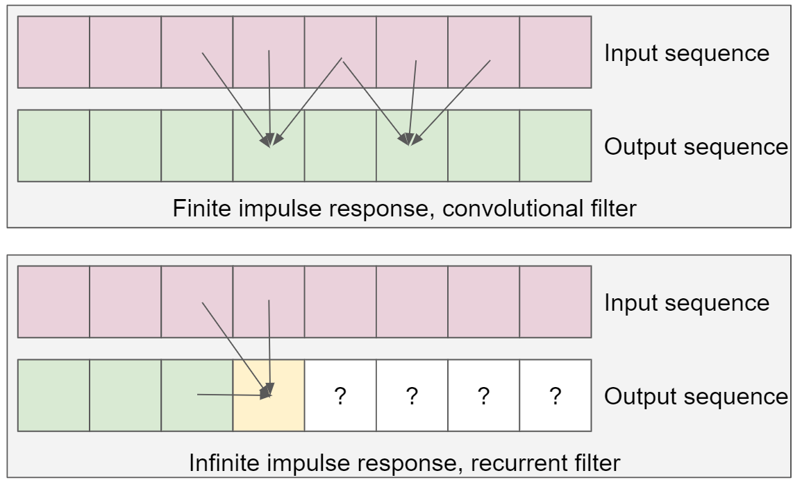
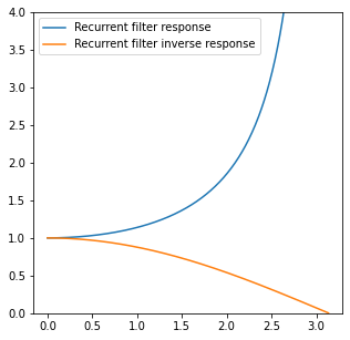
$x_0 = 2y_0 - x_{-1}$

This is already our final solution and a formula for a recurrent filter!

A recurrent filter (Infinite Impulse Response) is a filter in which each sequence value depends on the recurrent filter’s current and past inputs and outputs.

Here is a simplified diagram that demonstrates the difference:

Diferrence between Finite Impulse Response (convolutional) and Infinite Impulse Response (recurrent) filters.

In the above diagram, we observe that in an IIR filter to compute a “yellow” output element, we need the value of the previous output elements in the sequence. This contrasts with a finite impulse response filter – where the output depends only on the inputs, has no output dependence, and we can efficiently process them in parallel.

Implementing an IIR filter and some basic properties

If we were to write such a filter in Python, running it on an input list would be simple for loop:

def recurrent_inverse(seq):
    prev_val = seq[0]
    output = []
    for val in seq:
        output.append(2 * val - prev_val)
        prev_val = output[-1]
    return output

We need to initialize the first previous value to “something,” which depends on the used boundary conditions – often, initializing with the first value of the sequence is a reasonable default.

The recurrent filter has some interesting properties. For example, if we plot its impulse response, we get an infinite, oscillating one (hence the name “infinite impulse response”):

An impulse response of a recurrent filter deconvolving [0.5, 0.5] convolutional filter – truly infinite!

This filter’s frequency response and its inverse are a perfect inversion of the [0.5, 0.5] filter:

Frequency response of a recurrent filter deconvolving [0.5, 0,5] and its inverse.

The infinite response has a consequence of blowing up the Nyquist frequency to infinity – which we expected, as we are inverting a filter with zero response. If you process a signal consisting purely of Nyquist like:

$[1, 0, 1, 0, 1, 0, ...]$

The result is growing towards oscillating infinity:

$[1, -1, 3, -3, 5, -5, ...]$

This is the first potential problem of IIR filters – instability resulting from the signal processing concept of “poles.” Suppose the processed signal contains unexpected data (like frequencies not supposed to be present from the blurring). In that case, the result can be an infinite singularity and very quickly overflow numerically!

While I have solved this equation “by hand,” it’s worth noting that there is a neat linear algebra solution and connection. If we look at the convolution matrix, it’s… lower triangular matrix, and we can compute the solution with Gaussian elimination. This will come in handy in a later section.

Signal processing solutions

If you are interested in finding analytically inverse filters to any “arbitrary” system comprised of FIR and IIR filtering components, I recommend grabbing some dense signal processing literature. 🙂 The keywords to look for are Z-transform and “inverse Z-transform.”
The idea is simple: we can write a system’s response using a Z-transform. Then, some semi-analytical solutions (often involving circular integrals) compute a system with the exact inverse response. Those methods are not very easy and require quite a lot of theoretical background – and to be honest, I don’t expect most graphics engineers to find them very useful. Nevertheless, it’s a fascinating field that helped me solve many problems throughout my career.

The beauty of IIR filters

IIR filters (sometimes called in literature “digital filters,” which is somewhat confusing terminology for me) have the beautiful property of being exceptionally computationally sparse and efficient.

This simple box filter [0.5, 0.5] is complicated to deconvolve using FIR filters – even if we regularize its response to avoid “exploding” to infinity and an infinitely large filter footprint.

Here is an example of inverse, regularized / windowed FIR filter impulse response as well as its frequency response:

Truncated and windowed IR of a “deconvolving” IIR filter and its inverse frequency response. Even with 17 samples, the response has “ripples” and doesn’t achieve proper amplification of the highest frequencies.

I have used (my favorite) Hann window. Even with 17 taps of a filter, the resulting frequency response oscillates and doesn’t fully invert the original filter.

Note: truncating and windowing IIR filter responses is another practical way of finding desired deconvolving FIR filters analytically. I didn’t cover it in my original post (as it requires multiple steps: finding an inverse IIR filter and then truncating and windowing its response), but it can yield a great solution.

Comparing those 17 samples to just two samples of an inverse IIR filter – one past value, and one current value – recurrent filter is significantly more efficient.

This is why IIR filters are so popular when we need strong lowpass or highpass filtering with low memory requirements and low computational complexity. For example, almost all temporal anti-aliasing and temporal supersampling use recurrent filters!

Temporal antialiasing often uses an exponential moving average with a history coefficient of 0.9.

The resulting impulse response and frequency response are:

An impulse response of a recurrent moving exponential average filter and its impulse response. Getting so “steep” lowpass filtering with just two samples is impossible with FIR filters.

To get a similar lowpass effect in TAA, like with a recurrent formulation, one would have to use forty history samples, warp all of them according to their motion vectors/optical flow, and weight/reject according to occlusions and data changes. Just holding 40 past framebuffers is infeasible cost memory storage-wise, not to mention the runtime cost!

When a single IIR filter is not enough…

So far, I have used a deceptively simple example of a causal filter – where the current value depends only on the past values (in the [0.5, 0.5] filter, which shifts the image by a half-pixel).

This is the most often used type of filter in signal processing, which comes from the analog, audio, and communication domains. Analog circuitry cannot read a signal from the future! And it’s very similar to the TAA use case, where the latency is crucial, and we produce a new frame immediately without waiting for future ones.

Unfortunately, this is rarely the case for the other filters in graphics like blurs, Laplacians, edge/feature detectors, and many others. We typically want a symmetric, non-causal filter – that doesn’t introduce phase distortions and doesn’t shift the signal/image.

How do we invert a simple, centered [0.25, 0.5, 0.25] binomial filter? The center value “has to” depend both on the “past history” and the “future history”…

Instead, we can… run a single IIR filter forward and then the same filter backward!

This is suggested in classic signal processing literature and has an interesting algebraic interpretation. When we consider a tridiagonal matrix, we can look at its LU decomposition and proceed to solve it with Gaussian elimination.

Figure source: “A fresh look at generalized sampling,” D. Nehab, H. Hoppe.

Those methods get complicated and mathematically dense, and I will not cover those. They also don’t generalize to more complex filters in a straightforward manner.

Instead, I propose to use optimization and solve it using data-driven methods.

We will find a pair of backward and forwards recurrent filters just relying on straightforward gradient descent.

The first forward pass will start deconvolving the signal (and slightly shift it in phase), but the real magic will happen after the second one. The second pass not only deconvolves perfectly but also undoes any signal phase shifts:

Common solution to avoid phase shifts of recurrent filters is to run them twice – once forward and once backward. The second identical pass undoes any phase shifts of the first pass.

But first, let me comment on some reasons why it might not be the best idea to use an IIR filter in graphics and some of their disadvantages.

Why are IIR filters not more prevalent in graphics?

IIR filters are one of those algorithms that looks great in terms of theoretical performance – and in many cases, are genuinely performant. But also, it’s one of those algorithms that start to look less attractive when we consider a practical implementation – with implications like limited precision (both in fixed point and in floating point) and the usage of caches and memory bandwidth.

Let’s have a look at some of those. This is not to discourage you from using IIR filters but to caution you about potential pitfalls. This is my research and work philosophy. Think about everything that could go wrong and the challenges along the way. Determine if they could be solved – typically, the answer is yes! – and then confidently proceed to solve them one by one.

Instability

We have already observed how a simple recurrent filter inverting a [0.5, 0.5] convolutional filter can “explode” and go towards infinity on an unexpected sequence of data (frequency content around Nyquist).

In practice, this can happen due to user error, wrong data input, or a very unlucky noise pattern in the sequence. We expect algorithms not completely to break down on an incorrect or unfortunate data sequence – and in the case of IIR filter, even a localized error can have catastrophic consequences!

Imagine the accumulator intermittently becoming floating point infinity or “not a number” value. Then every single future value in the sequence depends on it and will also be corrupted – errors are not localized!

Such an error often occurs in many TAA implementations – where a single untreated NaN pixel can eventually corrupt the whole screen. On “God of War” we were getting QA and artist bug reports that were mysteriously named along the lines of “black fog eats the whole screen.” 🙂

Fixed point implementations generally tend to be more robust in that regard – as long as the code correctly checks for any potential over- or underflows.

Sensitivity to numerical precision

IIR filters rely on the past outputs – thus, any rounding error present in the previous computation might also accumulate, increasing – and eventually potentially “exploding” over time.

Here is an example:

Recurrent filters tend to accumulate any error and tend to deteriorate or completely lose stability over time.

This can be an issue with both fixed and floating point implementations.

This type of error is also highly data-dependent. On one input, the algorithm might perform perfectly, while on another one, the error can become catastrophic.

This is challenging for debugging, testing, and creating “robust” systems.

Limited data parallelism

IIR filters are considered “unfriendly” to a GPU or SIMD CPU implementation. When we process data at the time stamp N, we need to have computed the past values – which is an inherently serial process.

There are efficient GPU or SIMD implementations of the recurrent filters. Those typically rely on either vectorizing along a different axis (in an image, computing the IIR along the x-axis still allows for parallelism on the y-axis), splitting the problem into blocks, and performing most computations in the local memory.

This is significantly more difficult – especially on the GPU – than an FIR filter which can perform close to the performance limits – often even naively computed!

Multiple, transposed passes over data

Finally, the method for bidirectional IIR filters we are going to cover in the next section requires passing over the data in two passes – forward and backward. For separable filtering in 2D, this becomes four passes on both axes.

Even if every pass has minimal amounts of computations, this results in high memory bandwidth cost. By comparison, even large FIR filters – like 21×21 or even more, can go through the data in only a single pass. This matters especially on GPU when using an efficient compute shader or CUDA implementation, which can be extremely fast. This is one of the reasons why the machine learning world switched from recurrent neural networks to using attention layers and transformers for modeling temporal sequences like language or even video.

In image processing, one paper presented an interesting and smart alternative to bilateral filters for tasks like detail extraction or denoising – using recurrent filters for approximating geodesic filtering. Geodesic filters have different properties from bilateral ones and can be desirable in some tasks. Unfortunately, implementation difficulties, complexity of the technique, and performance made it somewhat prohibitive for its intended use (at least on mobile phones).

Data-driven IIR filter optimization

I present an alternative, much more straightforward way of finding a bi-directional recurrent filter that doesn’t require signal processing expertise.

Note: This section and the rest of the post assume the reader is familiar with “optimization” techniques that formulate an objective and solve it using iterative methods like gradient descent. If you are not familiar with those, I recommend reading my post on optimization first. It also introduces Jax as an optimization framework of my choice.

We formulate an optimization problem:

Start with some data sequence. Initially, a purely random “white noise” as it contains all the signal frequencies – later, we will analyze the impact of this choice. We will call this target sequence.
Apply the convolutional filter you would like to invert to the target sequence. We will call the resulting data input sequence.
Write a differentiable implementation of a recurrent filter and a function that runs it on the input data in both directions (forward and backward).
Create a differentiable loss function – for example, L2 – between the applied filter on the input sequence and the target sequence. The used loss function will strongly affect the results.
Initialize IIR parameters to an “identity” filter.
Run multiple iterations of gradient descent on the loss function with regard to the filter parameters. I used simple, straightforward gradient descent, but a higher order method and a dedicated optimizer can perform better.
After the optimization converges, we have our bidirectional recurrent filter!

Let’s go through those step by step – but if the concept doesn’t seem familiar, I recommend checking my past blog post on using offline optimization in graphics.

Similar to my past posts, I will use Python and Jax as my differentiable programming framework of choice.

Target and input sequences

This is the most straightforward step. Here is the target sequence (random, Gaussian noise), and an input sequence, convolved with a [1/4, 1/2, 1/4] “binomial” filter, for example:

Our training data – input and the optimization target.

Differentiable IIR filter and loss function

This part is not obvious – how to do it efficiently and generalize to any number of input and recurrent coefficients. I came up with this implementation:

def unrolled_iir_filter(x: jnp.ndarray, a: jnp.ndarray, b: jnp.ndarray) -> jnp.ndarray:
    if len(b) == 0:
        b = jnp.array([0.0])
    padded_x = jnp.pad(x, (len(a) - 1, 0), mode="edge")
    output = jnp.repeat(padded_x[0], len(b))
    for i in range(len(padded_x) - len(a) + 1):
        aa = jnp.dot(padded_x[i : i + len(a)], a)
        bb = jnp.dot(output[-len(b) :], b)
        output = jnp.append(output, aa + bb)
    return output[-len(x) :]

This is not going to be super fast, but if we need it, Jax allows us to both jit and vectorize it over many inputs.

Application and the loss function are very straightforward, though:

@jax.jit
def apply(x, params):
    first_dir = unrolled_iir_filter(x[::-1], params[0], params[1])
    return unrolled_iir_filter(first_dir[::-1], params[0], params[1])
 
@jax.jit
def loss(params):
    padding = 5
    return jnp.mean(jnp.square(apply(test_signal, params) - target_signal)[padding:-padding])

The only thing worth mentioning here is that I compute the loss ignoring the boundaries of the result as the boundary conditions applied there can distort the results.

Optimize!

Having everything set up, we run our gradient descent loop. It converges very quickly; I run it for 1000 iterations, taking a few seconds on my laptop. This is how the optimization progresses:

And here is the result, almost perfect!

Optimization result – close to perfect deconvolution.

This closeness is remarkable because we cannot recover “some” frequencies (the ones close to Nyquist that get completely zeroed out).

The recurrent filter values I got are 1.77 for the current sample and -0.75 for the past output sample. It’s worth noting that there is an error from the optimization process – those don’t sum to 1.0, but we can correct it easily (normalize the sum). Running the optimization procedure on a larger input would prevent the issue.

When we compute and plot an impulse response of this filter, we get:

The impulse response of the IIR filter – first pass in orange and both passes combined in blue.

I have plotted two IRs: one after passing through the IIR in the forward direction and then after the backward direction pass.

We observe how the second pass simultaneously symmetrizes the filter and makes the response significantly “stronger,” with much larger oscillations. We can explain the effect of symmetrizing and undoing the phase shifts intuitively – the filter applies the same shifts in the opposite direction – which cancels them out.

Do you have an intuition about the frequency response of the two-pass filter? The frequency response of two passes is the response squared of a single pass:

The frequency response of two passes is the frequency response of a single pass squared.

This comes from the duality of convolution / linear filtering in the spatial domain and multiplication in the frequency domain.

Here is again the demo of this filtering process happening on an actual signal, first the forwarded pass and then the backward pass:

Animation showing deconvolution and recurrent filtering progress.

With two passes, each taking just two samples, we got a recurrent filter equivalent to ~128 samples FIR filter and a squared response of a single recurrent filter!

Plotting the also the inverse response of the combined filter, we get close to the perfect inversion of the [0.25, 0.5, 0.25] filter:

Regularizing against noise

The above response is extreme; it doesn’t go to an infinite boost of the Nyquist frequencies, but in this example, the amplification is ~300. Under the tiniest amount of imprecision, quantization, or noise, it will produce extremely noisy results full of visual artifacts.

Luckily, in this data-driven paradigm regularizing against the noise is as simple as adding some noise before starting the filter coefficient optimization.

test_signal += np.random.normal(size=test_signal.shape) * reg_noise_mag

Regularizing the training data by adding noise results in regularized, weaker deconvolving filters that avoid amplifying the noise too much.

This also caps the maximum frequency response at ~9x boost:

Regularized filter’s frequency response and its inverse.

We observe that this regularization smoothens the deconvolution results as well:

Regularized deconvolution doesn’t restore all highest frequencies.

What would happen when the noise becomes of a similar magnitude to the original signal?

Very strong regularization (by adding a lot of noise to the input sequence) results in a smoothing and denoising filter with no deconvolution properties!

The data-driven approach automatically learns to get a lowpass, smoothing/denoising filter instead of a deconvolution filter! This can be both a blessing and a curse. Data-adaptive behavior is desirable for practical systems (when the theoretical assumptions and models can be simply wrong). Still, it can lead to surprising behaviors, like wondering, “I asked for a deconvolution filter, not a lowpass filter, this makes no sense.”

Why is the resulting filter lowpass, though, if the noise was 100% white and should contain “all” frequencies? This comes from the per-frequency signal-to-noise ratio. After adding noise to a blurred signal, SNR in those highest frequencies is very close to zero; an optimal filter will remove it. In the lower frequencies (not affected by blur), the amount of noise in proportion to the signal is lower. Thus we need less denoising of those lower frequencies. In my previous post, I described Wiener deconvolution which is an analytical solution that explicitly uses the per-frequency signal-to-noise ratio.

Signal- and data-dependent optimal deconvolution

This naturally brings us to another advantage of data-driven filter generation and optimization. We can use “any” data, not just white noise; more importantly – data that resembles the target use case.

Real data distribution doesn’t look like white noise. For instance, natural images contain significantly more of the lowest frequencies (which is why image downsampling removes detail but can be extreme and we can still tell the image contents).

Similarly, audio signals like speech have a characteristic dominating frequency range of around 1kHz, and our auditory system is optimized for it.

A linear deconvolution filter that is L2-optimal for “natural” images might be very different from the one operating on the white noise! Let’s test this insight.

We will test the original white noise signal with a very subtly filtered version of it (reduced “high shelf” to remove some of the highest frequencies):

Training data that doesn’t follow a perfect “white noise” all frequency spectrum.

After optimizing test signals (both target signals filtered with [0.25, 0.5, 0.25]), we get radically different results and filters:

Using slightly different training data we get dramatically different resulting impulse and frequency responses!

The difference is huge! Even more significant than the one from simply the noise regularization – which might be surprising considering how visually similar both training examples are.

The filter learned on non-white noise is milder and will not create severe artifacts from mild noise or quantization. Its significantly smaller spatial support won’t lead to as noticeable ringing – and won’t “explode” when applied to signals with too much high frequency content.

On the other hand, our perception is very non-linear. Despite images containing not many high frequencies, we are very sensitive to the presence of edges – and an L2 optimized filter ignores this. This is why it is important to model both the data distribution and the loss function correctly representing the task we are solving.

This lesson keeps reappearing in anything data-driven, optimization, and machine learning. Your learned functions, parameters, and networks are only as good as the training data and the loss function match of the real-world target data and the task being solved. Any mismatch will create unexpected results and artifacts or lead to solutions that “don’t work” outside of the publication realms.

Moving to 2D

So far, my post has focused on 1D signals for ease of demonstration and implementation.

How can one use IIR on 2D images?

Suppose you have a separable filter (like Gaussian). In that case, the solution is simple – running the filter four times – back and forth on the horizontal axis and then on the vertical axis (this generalizes to 3D or 4D data).

Here is a visual demonstration of this process:

Efficiently implementing this on a GPU is not a trivial task – but definitely possible.

Non-separable filters are not easy to tackle – but one can fit a series of multi-pass, different IIR filters. I posted about approximating non-separable shapes with a series of separable filters; here, the procedure would be analogous and automatically learned.

Alternatively, it’s also possible to have a recursion defined in terms of the previous rows and columns. I encourage you to experiment with it – in a data-driven workflow, one doesn’t need decades of background in signal processing or applied mathematics to get reasonably working solutions.

Summary

IIR filters can be challenging to work with. They are sensitive, easily become unstable, are hard to optimize and implement well, require multiple passes over data, and don’t trivially generalize to non-separable filters and 2D.

Despite that, recurrent filtering can have excellent compactness and efficiency – especially for inverting convolutional filters and blurs. They are the bread-and-butter of any traditional and modern audio and signal processing. Without them, graphics’ temporal supersampling and antialiasing techniques wouldn’t be as effective.

In this post, I have proposed a data-driven, learned approach that removes some of their challenges. When learning an IIR filter, we don’t need to worry about complicated algebra and theory, noise, or signal characteristics – and the code is almost trivial. We obtain an optimal filter in a few thousand fast gradient descent iterations. Mean squared error (or any other metric, including very exotic ones, as long as they are differentiable) can define optimality.

The next step is making those learned filters non-linear, and there are numerous other fascinating uses of data-driven learning and optimization of “traditional” techniques. But those will have to wait for some future posts!

Posted in Code / Graphics | Tagged algorithms, digital signal processing, graphics, graphics programming, image processing, jax, maths, numpy, python, signal processing | Leave a comment

Progressive image stippling and greedy blue noise importance sampling

Posted on August 31, 2022 by bartwronski

Introduction

I recently read the “Gaussian Blue Noise” paper by Ahmed et al. and was very impressed by the quality of their results and the rigor of their method.

They provide a theoretical framework to analyze the quality of blue noise from a frequency analysis perspective and propose an improved technique for generating blue noise patterns. This use of blue noise is very different from “blue noise masks” and regular dithering – about which I have a whole series of posts if you’re interested.

Authors of the GBN paper show some gorgeous blue noise stippling patterns:

Source: “Gaussian Blue Noise,” Ahmed et al.

Their work is based on an offline optimization procedure and has inspired me to solve a different problem – progressive stippling. I thought it’d look super cool and visually pleasing to have some “progressive” blue-noise stippling animations from an image.

By progressive, we mean creating a set of N sample sets, where:

each one has 1…N samples,
a set K is a subset of the set K+1 (set K+1 adds one more point to the set K),
each set K fulfills the blue noise criterion.

By fulfilling all three criteria (especially the second), the “quality” (according to the third) of the last complete set cannot be as high as in, for example, the “Gaussian Blue Noise” paper. In optimization, every new constraint and additional requirement sacrifices other requirements.

We won’t have as excellent blue noise properties as in the cited GBN paper, but as we’ll see, we can get “good enough” and visually pleasing results.

Progressive sampling is a commonly used technique in Monte Carlo rendering for reconstruction that improves over time (critical in real-time/interactive applications) but less commonly in stippling/dithering – I haven’t found a single reference to progressive stippling.

Here, I propose a straightforward method to achieve this goal.

Method

As a method, I augment my “simplified” variation of the greedy void and cluster algorithm with a trivial modification to the initial “energy” potential field.

Instead of uniform initialization, I initialize it with the image intensity scaled by some factor “a.”

(Depending on the type of stippling, with black “ink” dots or with the bright “light splats,” you might want to “negate” this initialization)

Factor “a” will balance the image content’s importance compared to filling the whole image plane with the blue noise distribution property.

In my original implementation, the Gaussian kernel used for energy modification was unnormalized and didn’t include a correction for small sigma. I fixed those to allow for easier experimentation with different spatial sigmas.

One should consider the boundary conditions for applying the energy modification function (zero, mirror, clamp) for the desired behavior. For example, spherically-wrapped images like environment maps should use “wrap” while displayable ones might want to use “clamp.” I ignore it here and use the original “wrap” formulation, suitable for use cases like spherical images.

We stop the iteration after we reach the desired point count – for example, equal to the average brightness of the original image.

This is the whole method!

Here is the complete code:

def gauss_small_sigma(x: np.ndarray, sigma: float):
    p1 = scipy.special.erf((x - 0.5) / sigma * np.sqrt(0.5))
    p2 = scipy.special.erf((x + 0.5) / sigma * np.sqrt(0.5))
    return (p2 - p1) / 2.0
 
 
def void_and_cluster(
    input_img: np.ndarray,
    percentage: float = 0.33,
    sigma: float = 0.9,
    content_bias: float = 0.5,
    negate: bool = False,
) -> Tuple[np.ndarray, np.ndarray]:
    size = input_img.shape[0]
 
    wrapped_pattern = np.hstack((np.linspace(0, size / 2 - 1, size // 2), np.linspace(size / 2, 1, size // 2)))
    wrapped_pattern = gauss_small_sigma(wrapped_pattern, sigma)
    wrapped_pattern = np.outer(wrapped_pattern, wrapped_pattern)
    wrapped_pattern[0, 0] = np.inf
 
    lut = jnp.array(wrapped_pattern)
    jax.device_put(lut)
 
    def energy(pos_xy_source):
        return jnp.roll(lut, shift=(pos_xy_source[0], pos_xy_source[1]), axis=(0, 1))
 
    points_set = []
 
    energy_current = jnp.array(input_img) * content_bias * (-1.0 if negate else 1.0)
    jax.device_put(energy_current)
 
    @jax.jit
    def update_step(energy_current):
        pos_flat = energy_current.argmin()
        pos_x, pos_y = pos_flat // size, pos_flat % size
        e = energy_current[pos_x, pos_y]
        return energy_current + energy((pos_x, pos_y)), pos_x, pos_y, e
 
    final_stipple = np.zeros_like(lut) if negate else np.ones_like(lut)
 
    samples = []
    for x in range(int(input_img.size * percentage)):
        energy_current, pos_x, pos_y, e = update_step(energy_current)
        samples.append((pos_x, pos_y, input_img[pos_x, pos_y]))
        final_stipple[pos_x, pos_y] = 1.0 if negate else 0.0
    return final_stipple, np.array(samples)

And it works pretty well:

With different factors “a,” we get the different balancing of filling the overall image space more as contrasted to a higher degree of importance sampling with the equal sample count:

Different factors “a”, balancing preference for blue noise vs importance sampling.

When the parameter goes towards infinity, we get the pure progressive sampling of the original image. The other extreme will produce pure blue noise, filling space and ignoring the image content:

The behavior of low values is interesting. With the increasing point count, they first reveal the shape, then give a ghostly “hint” of the shape underneath, and finally turn into almost uniform spatial filling:

Different sample counts for low preference for image contents (and high for preserving blue-noise space filling).

Why does this work?

Results look pretty remarkable, given the straightforward and almost “minimal” method, so why does it work?

When we initialize the energy field with the image, we find the brightest/darkest point (depending on whether we negated the image content) as the one with minimum energy. After the first update, we add energy to this position. The next iteration finds and updates a different point. Here is a visualization (slightly exaggerated) for 1, 2, 11, and 71 points:

Each iteration both excludes the point from being reprocessed (sets it as “infinite energy”) as well as produces a Gaussian “splat” that makes the points around it less desirable to be “picked” in the following close iterations. The algorithm will choose something further away from it. The “a” constant and the Gaussian sigma balance the repulsion of points with the priority of the pixel intensity.

Edge sampling

When stippling, classic literature (ref1 ref2) emphasizes how the stippling of the edges is more critical than stippling the constant areas – both for “artistic” reasons and because the human visual system has strong edge detection mechanisms.

The above example worked very well for two reasons.

The most important secret was that Kodak images – like most images on the internet – are sharpened for display and printing. If you look at the boat paddle in the picture, you will notice a bright halo around it. Almost all images have sharpening, tiny halos, and gradient reversals.

The second reason relates to the method: looking at single points in combination with blue noise like “repulsion” will push many points to the edges.

But if we look at the simplest analytical unsharpened example – a circle, we find that the shape is somewhat visible, but not overly so:

When the image is very simple and has only some edges, the shape after blue-noise stippling can be only barely visible.

The solution is straightforward, and along the lines of observation of sharpened internet images, we can pre-sharpen the image arbitrarily (just before generating the initialization energy).

The amount of sharpening determines how strong we are going to reproduce the edges:

Visualization of blue-noise stippling after applying different sharpening factors.

All of the above are very usable, and I like it the most and find it the most useful when our constant “a” is low (biasing the results towards preserving space-filling blue-noise properties more than contents brightness). Visible edges can make a huge difference in how we perceive low-contrast shapes.

Improving the final state further

The suboptimality of the described method at the final state can be improved slightly (at the cost of breaking the progressive results) by “fine-tuning” the positions of points based on the last point set and according to the energy defined like in the GBN paper. However, one would have to allow it not to go too far from the original positions to preserve the progressive property.

This approach is not unlike standard methods in deep learning, where one fine-tunes the training/optimization results on specific, more relevant examples – typically using fewer iterations and a slower learning rate to avoid over-fitting.

Use for importance sampling

The use-case I have described so far is… cute and produces fun and pretty animations, but can it be useful? Probably the concept of “progressive stippling” – not so much beyond artistic expression.

But if we squint our eyes, we make the following observations:

Thanks to the “progressive” property, points are sorted according to “importance,”
Importance consists of two components:
1. Blue noise spatial distribution,
2. The value of the input pixel.
We don’t have to stop at the average brightness and can continue until we fill all the points.

Note, however, that the sorting/importance is not according to just the brightness or good spatial distribution; it’s a hybrid metric that combines both and depends on the spatial relationships and distribution.

Could we use it for blue noise distributed importance sampling of images?

Importance sampling of images is commonly used for evaluating image-based lighting or sampling 2D look-up tables for terms we lack analytical solutions. Most approaches rely on complicated spatial division structures built offline and traversed during the sampling process.

I propose to use the sorted progressive stippling points (and their pixel values) in the importance sampling process.

Let’s use a different Kodak image, a crop of the lighthouse (and inverting for the sampling of the brights):

An inverse-stippled different image from the Kodak dataset.

If we plot the brightness of the consecutive points in the sequence, we observe it is a very “noisy” version and distorted version of the image histogram:

Progressive point brightness values, values smoothened, and the actual normalized image histogram.

The distortion is non-obvious, hard to predict, and depends on the spatial co-locality of the points in the image. Different images with identical histograms will get different results based on where the similarly valued pixels are.

To use it in practice for importance sampling, I propose to use a smoothened, normalized version of this histogram as a PDF. Based on the inverse-sampled value, pick a point from the sequence. The sample stores information about its intensity and the original location in the image.

For simplicity’s sake and a quick demonstration, I will use an ad-hoc inverse CDF of exponentiating a random number to the power of 3 (equivalent to $\frac{1}{3x^{\frac{2}{3}}} PDF).

For example, with the uniform random variable value of 0.1, we will pick 0.1**3 == 0.001 percentile point from the progressive stippling sequence.

The following figure presents what the four different batches of 1000 random samples from this distribution look like:

Blue-noise greedy importance sampling – 4 different realizations of 1000 random samples.

And by comparison, the same sample counts, but with pure importance sampling based on the image brightness:

White noise importance sampling produces significantly more “clumping”.

The latter has significantly more “clumping” and worse space coverage outside bright regions. This difference might matter for the cases of significant mismatch of the complete integrand (often a product of multiple terms) with the image content.

Many small details are necessary to make this method practical for Monte Carlo integration. A pixel’s fixed (x, y) position is not enough to sample other terms appearing in an actual Monte Carlo integral, like a continuous PDF of a BRDF. One obvious solution would be to perform jittering within pixel extents based on additional random variables.

I don’t test the effectiveness of this method. I believe it would give less variance at low sample counts but not improve the convergence (this is typical with blue noise sampling).

Finally, this method can be expanded to more than just two dimensions – as long as we have a discrete domain and can splat samples into it.

But I leave all of the above – and evaluation of the efficacy of this method to the curious reader.

Conclusions

I have presented an original problem – progressive stippling of images and a method to compute it with a few lines of code of modification of the “void and cluster” blue noise generation method.

It worked surprisingly well, and I consider it a fun, successful experiment, just look again at those animations:

It seems to have some applications beyond fun animations, like very fast blue-noise preserving importance sampling of textures, environment maps, and look-up tables. I hope it inspires some readers to experiment with that use case.

Posted in Code / Graphics | Tagged algorithms, blue noise, dithering, graphics, graphics programming, image processing, jax, programming, python, sampling | 3 Comments

Removing blur from images – deconvolution and using optimized simple filters

Posted on May 26, 2022 by bartwronski

**Left:** Original image. **Center:** Blurred through convolution. **Right:** Deconvolution of the blurred image.

In this post, we’ll have a look at the idea of removing blur from images, videos, or games through a process called “deconvolution”.

We will analyze what makes the process of deblurring an image (blurred with a known blur kernel) – deconvolution – possible in theory, what makes it impossible (at least to realize “perfectly”) in practice, and what a practical middle ground looks like.

Simple deconvolution is easy to understand, and it connects very nicely pure intuition, linear algebra, as well as frequency domain and spectral matrix analysis.

In the second part of the post we will look at how to apply efficient approximate deconvolution using only some very simple and basic image filters (gaussians) that work very well in practice for mild blurs.

Linear image blur – convolution

Before we dive into defining what is “deblurring” (or even going further into deconvolution), let’s first have a look at what is blur.

I had posts about various kinds of blurs, the most common being Gaussian blur.

Let’s stop for a second and look at the mathematical formulation of blur through convolution.

Note: I will be analyzing mostly examples in 1D dimension, calling sequence entries “samples”, “elements”, and “pixels” interchangeably, while also demonstrating image convolutions as 2D (separable) filters. 2D is a direct extension of all the presented concepts in 1D – harder to visualize in algebraic form or frequency plots, but more natural for looking at the images. I hope examples in alternating 1D and 2D won’t be too confusing. Separable filters can be deconvolved separably as well (up to a limit), while non-separable ones not.

“Blur” in “blurry images” can come from different sources – camera lens point spread function, motion blur from hand shake, excessive processing like denoising, or upsampling from lower resolution.

All of those have in common that come from a filter that either “spreads” some information like light rays across the pixels, or alternatively combines information from multiple source locations (whether physical circle of confusion, or nearby pixels). We typically call it a “blur” when all weights are positive (this is the case in physical light processes, but for electric or digital signals not necessarily), and it results in a low-pass filter.

There are two mentioned ways of looking at blurs – “scatter”, where a point contributes into multiple target output elements, and “gather”, where for each destination elements, we look at contributing source points. This is a topic for a longer post, but in our case – where we look at “fixed” blurs shared by all the locations in the image – they can be considered equivalent and transpose of one another (if a source pixel contributes to 3 output pixels, each output pixel also depends on 3 input pixels).

Let’s look at one of the simplest filters, binomial convolution filter [0.25, 0.5, 0.25].

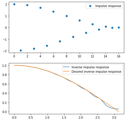
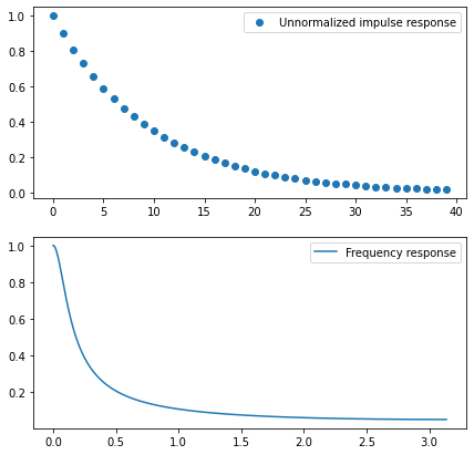
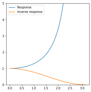
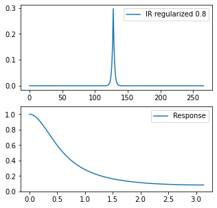
This filter means that given five pixels, , we have output pixels:

Note that for now we have omitted the output pixels and it’s not immediately obvious how to treat them; where would we get the missing information from (reading beyond )? This relates to “boundary conditions” which matter a lot for analysis and engineering implementation details, and we will come back to it later. Typical choices for “boundary conditions” are wrapping around, mirroring pixels, clamping to the last value, treating all missing ones as zeros, or even just throwing away partial pixels (this way a blurred image would be smaller than the input).

In physical modeling – for example when blur occurs in camera lens – we sample a limited “rectangle” of pixels from a physical process that happens outside, so it’s similar to throwing away some pixels.

Such a simple [0.25, 0.5, 0.25] filter and simple convolution when applied on an image in 2D (first in 1D in horizontal axis and then in 1D in the vertical one, results in a relatively mild, pleasant blur:

**Left:** Original image crop. **Right:** Blurred.

But if we had such an image and we knew where the blur comes from and its characteristics… could we undo it?

Deblurring through deconvolution

Process of inverting / undoing a known convolution is called simply deconvolution.

We apply a linear operator to the input… so, can we invert it?
In a fully general case not always (general rules of linear systems apply; not all are invertible!), but “approximately”? Most often yes, and let’s have a look at the math of deconvolution.

But before that, I will clarify a common confusing topic.

Is deconvolution the same as sharpening, super-resolution, upsampling?

No, no, and no.

Deconvolution – process of removing blur from an image.

Sharpening – process of improving the perceived acuity and visual sharpness of an image, especially for viewing it on a screen or print.

Super-resolution – process of reconstructing missing detail in an image.

Upsampling – process of increasing the image resolution, with no relation to blur, sharpness, or detail – but aiming to at least not reduce it. Sadly ML literature calls upsampling “single frame super-resolution”.

Where does the confusion come from?

Other than the ML literature super-resolution confusion, there is overlap between those topics. Sharpening can be used to approximate deconvolution and often provides reasonable results (I will show this around the end of this post). If you did sharpening in Photoshop to save a blurry photo, you tried to approximate deconvolution this way!

Super-resolution is often combined with deconvolution in “CSI” style detail and acuity enhancement pipelines.

Upsampling is often considered “good” when it produces edges with sharper falloff than the original Nyquist and often has some non-linear and deconvolution-like elements.

But despite all that, deconvolution is simply undoing a physical process or pipeline processing of a convolution.

Equations of deconvolution

Let’s have a look at the equations that formed the basis of convolution again:

It should be obvious that we cannot directly solve for any of x variables – we have 3 equations and 5 unknowns…

But if we look at some simple manipulation:

We can see that we get:
, where is a residual error (sum of four quartered input pixels)

If we apply this filter to the blurred image from before we get… an ugly result:

**Left:** Original image. **Center:** Blurred through convolution. **Right:** Our first, failed attempt at deconvolution.

Yes, it is very “sharp”, but… ugh.

It’s clear that we need more “source” data. We need “something” to cancel out those error terms further away…

Note: I did this exercise, as this is important to build intuition and worth thinking about – for full cancellation we will need more and more terms, up to infinity. Anytime we include pixels further away, we can make the residual error smaller (as multiplying by the further weights and iterating this way shrinks them down).

But to solve an inverse of a linear system in general – we obviously need at least as many knowns as unknowns in our system of equations. At least, because linear dependence might make some of those equations cancel out.

This is where boundary conditions and handling of the border pixels comes into play.

One example is “wrap” mode, which corresponds to circulant convolution (we will see in a second why this is neat for mathematical analysis; not necessarily very relevant for practical application though 🙂 ).

Notice the bolded “wrapping” elements. I was too lazy to solve it by hand, so I plugged it into sympy and got:

This is a valid solution only for this specific, small circulant system of equations. In general, we could definitely end up with a non-invertible system – where we lose some degrees of freedom and again have too many unknowns as compared to known variables.

But in this case, if we increase the number of the pixels to 7, we’d get:

There’s an interesting pattern happening… that pattern (sign flipping and adding plus two to a center term) will continue – to me this looked similar to a gradient (derivative) filter and it’s not a coincidence. If you’re curious about the connection, check out my past post on image gradients and derivatives and have it in mind once we start analyzing the frequency response and seeing the gain for the highest frequencies going towards infinity.

For the curious – if we apply such a filter to our image, we get absolutely horrible results:

**Left:** Original image. **Center:** Blurred through convolution. **Right:** Our second, even more failed attempt at deconvolution.

This got even worse than before.

Instead of toying with tiny systems of equations and wondering what’s going on, let’s solve it by getting a better understanding of the problem and going “bigger” and more general: looking at the matrix form of the system of equations.

Convolution and deconvolution matrix linear algebra

Any system of equations can be represented in a matrix form.

Circulant convolution of 128 pixels will look like this:

1D signal [0.25 0.5 0.25] circulant convolution matrix.

Make sure you understand this picture. Horizontal rows are output elements, vertical columns are input elements (or vice versa; row major vs column major, in our case it doesn’t matter, though I am sure some mathematicians would scream reading this). Each row has 3 elements contributing to it – in 1D each output element depends on 3 input elements.

This is a lovely structure – (almost) block diagonal matrix. Very sparse, very easy to analyze, very efficient to operate.

Edit: Nikita Lisitsa mentioned on twitter that this specific matrix is also tridiagonal. Those appear in other applications like 1D Laplacians and are even easier to analyze. More general convolutions (more elements) are not tridiagonal though.

Then to get a solution, we can invert the matrix (this is not a great idea for many practical problems, but for our analysis will work just fine). Why? This linear system transforms from input elements / pixels to output elements pixels. We are interested in the inverse transformation – how to find the input, unblurred pixels, knowing the output pixels.

However, if we try to invert it numerically… we get an absolute mess:

First attempt at inverting the convolution matrix.

Numpy produces this array: [[-4.50359963e+15, 4.50359963e+15, -4.50359963e+15, …,]]. When we look at the determinant of the matrix, it is close to zero, so we can’t really invert it. I am surprised I didn’t see any actual errors (numerical and linear algebra packages might or might not warn you about matrix conditioning). This means that our system is “underdetermined” (some equations are linearly dependent on each other and there is not enough information in the system to solve for the inverse) and we can’t solve it exactly…

Luckily, we can regularize the matrix inverse by our favorite tool – singular value decomposition. In the SVD matrix inversion, we obtain an inverse matrix by inverting pointwise singular values and transposing and swapping the singular vector matrices.

Singular values look like this:

If this reminds you of something… just wait for it. 🙂

But we see that we can’t really invert those singular values that are close to 0.0. This will blow up numerically, up to infinity. If we regularize the inversion (instead of do for example ), we can get a “clean” inverse matrix:

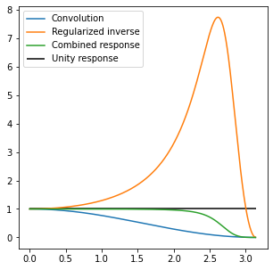
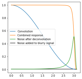
Regularized inverse of the convolution matrix.

This looks much more reasonable. And if we apply a filter obtained this way (one of the rows) to the blurred image,we get a high quality “deblurred” image, almost perfectly close to the source:

**Left:** Original image. **Center:** Blurred through convolution. **Right:** Proper deconvolution of the blurred image.

Worth noting: if we had a filter that does somewhat less blur, for example [0.2, 0.6, 0.2], we would get singular values:

Singular values of a milder filter convolution matrix.

And the direct inversion would be also much better behaved (no need to regularize):

Direct, non regularized inverse of the milder blurring convolution matrix.

Time to connect some dots and move to a more “natural” (and my favorite) convolution domain – frequency analysis.

Signal processing and frequency domain perspective

Let’s have a look at the frequency response of the original filter. Why? Because we will use Fourier transform and convolution theorem. It states that when performing (inverse or regular) Fourier transform (or its discrete equivalents) convolution in one space is multiplication in the other space.

So if we have a filter response like this:

(Looks familiar?)

It will multiply the original frequency spectrum. We can combine linear transforms in any order, so if we want to “undo” the blurring convolution, we’d want to multiply by… simply its inverse.

Here we encounter again the difficulty of inversion of such a response – it goes towards zero. To invert it, we would need to have a filter with response going towards infinity:

This would be a bad idea for many practical reasons. But if we constrain it (more about the choice of constraint / regularization later), we can get a “reasonable” combined response:

Inverting frequency response of a [0.25 0.5 0.25] filter with regularization.

We would like the “combined response” to be a perfect flat unity, but this is not possible (need for an infinite gain) – so something like this looks great. In practice, when we deal with noise, maximum gains of 8 might already be too much, so we would need to reduce it even more.

But before we tackle the “practicalities” of deconvolution, it’s time for a reveal of the connection between the matrix form and frequency analysis.

They are exactly the same.

This shouldn’t be surprising if you had some “advanced” linear algebra at college (I didn’t; and felt jealous watching Gilbert Strang’s MIT linear algebra course – even if you think you know linear algebra, whole course series is amazing and totally worth watching) or played with spectral analysis / decomposition (I have a recent post on it in the context of light transport matrices if you’re interested).

Circulant matrix, such as convolution matrix, diagonalizes as Discrete Fourier Transform. This is an absolutely beautiful and profound idea and analyzing behaviors of this diagonalization was one of the prerequisites for the development of the Fast Fourier Transform.

When I first read about it, I was mind blown. I shouldn’t be surprised – Fourier series and complex numbers appear everywhere. Singular values of a circulant (convolution) matrix are amplitude frequency buckets of the DFT.

This is the reason I picked kind of “unnatural” (for graphics folks) wrapping boundary condition – Fourier transform is periodic and a wrapping cyclic convolution matrix is diagonalized through it. We could have picked some other boundary conditions and the result would be “similar”, but not exactly the same. In practice, it doesn’t matter outside of the borders (where “mirror” would be my practical recommendation for minimizing edge artifacts for blurs; and either “mirror” or “clamp” works well for deconvolution).

This is another way of looking at why some convolution matrices are impossible to invert – because we get frequency response at some frequency buckets equal to zero and therefore the singular values also equal to zero!

Nonlinear, practical reality of deblurring

I hope you love convolution matrices and singular values as much as I do, but if you don’t – don’t worry, time to switch to more practical and applicable information. How can we make simple linear deconvolution work in practice? To answer that, we need to analyze first why it can fail.

Infinite gain

We already discovered one of the challenges. We cannot have an “infinite” gain on any of the frequencies. If some information from singular values / frequencies truly goes to 0, we cannot recover it. Therefore, it’s important to not try to and not invert the frequencies close to zero and constrain the maximum gain to some value. But how and based on what? We will see how noise helps us answering this question.

Noise

The second problem is noise. In photography, we always deal with noisy images and noise is part of the image formation.

If we add noise with standard deviation of 0.005 to the blurry image (assuming signal strength of 1.0), we’re not going to notice it. But see what happens when deconvolving it:

**Left:** Original image. **Center:** Blurred through convolution. **Right:** Deconvolution of a slightly noisy image.

This relates to the gain point before – except that we are not concerned with just “infinite” gains, but any strong gain on any of the frequency buckets will amplify the noise at that frequency… This is a frequency space visualization of the problem:

Amplification of noise happening because of the deconvolution.

Notice how the original white noise got transformed into some weird blue-noise (only the highest frequencies) – and we can see this actually on the image, with an extreme checkerboard-like pattern.

Quantization, compression, and other processing

Noise is not the only problem.

When processing signals in the digital domain, we always quantize them. While rendering folks might be working a lot with floats and tons of dynamic range (floats obviously also quantize, but it’s an often forgiving, dynamic quantization), unfortunately camera image signal processing chain, digital signal processors, and image processing algorithms mostly don’t. Instead they operate on fixed point, quantized integers. Which makes a lot of sense, but when we save an image in 8 bits (perfectly fine for most displays) and then try to deconvolve it, we get the following image:

**Left:** Original image. **Center:** Blurred through convolution. **Right:** Deconvolution of an 8-bit image.

The noise itself is not huge; but in terms of structure, it definitely is similar to the noisy one above – this is not a coincidence.

Quantization can be thought of as adding quantization noise to the original signal. If there is no dithering, this quantization noise is pretty nasty and correlated, with dithering it can be similar to white noise (with known standard deviation). In either case, we have to take it into account to not produce visual artifacts and one can use expected quantization noise standard deviation of , where is a difference between two closest elements due to quantization.

Significantly worse problems can arise from other image processing and storage techniques like compression. Typically a high quality deconvolution from compressed images is impossible using linear filters – but can be definitely achieved with non-linear techniques like optimization or machine learning.

Aliasing

And then, there’s aliasing. The ubiquitous signal processing and graphics problem. The reason it comes up here is that even if we model blur coming from a lens perfectly, then when we sample the signal by camera sensor and introduce aliasing, this aliasing corrupts the measurements of the higher (and sometimes mid or lower!) frequencies of the input signal.

This is beyond the scope of this post, but this is why one would want to do a proper super-resolution and multiframe reconstruction of the signal first – that both removes aliasing, as well as reconstructing the higher frequencies – before any kind of deconvolution. Unfortunately any super-resolution reconstruction error might be amplified heavily this way, so worth watching out.

Different signal space, gamma etc

If blur happens in one space (e.g. photons, light intensity), then deblurring in another space (gamma corrected images) is a rather bad idea. It can work “somewhat”, but I’d recommend against doing so. Interestingly, my recommendation is at odds with the common practice of sharpening (for appearance) in the output space (“perceptual”) which tends to produce less over-brightening – while convolution happens in the linear light space. I will ignore this subtlety here, and simply recommend deconvolving in the same space as the convolution happened.

Regularizing against noise and infinities

What can we do about the above in practice? We can always bound the gain to some maximum value and find it by tuning. That can work ok, but feels inelegant and is not noise magnitude dependent.

An alternative is Wiener deconvolution which provides a least-squares optimal estimation of the inverse of a noisy system. Generally, Wiener filter requires knowing the power spectral density distribution of the input signal. We could use the image / signal empirical PSD, or general, expected distribution for natural images. But I’ll simplify even further and assume a flat PSD of 1 (not correct for natural images that have a strong spectral decay!), getting a formula for a general setting with response of , where X is a convolution filter frequency response, and is per frequency noise standard deviation. Wikipedia elegantly explains how this can be rephrased in terms of SNR:

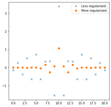
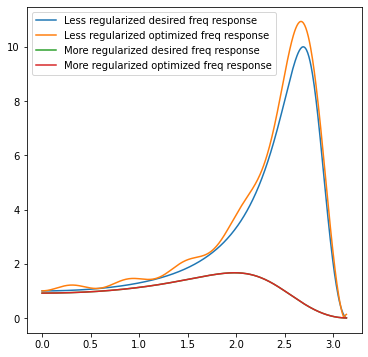
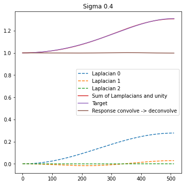
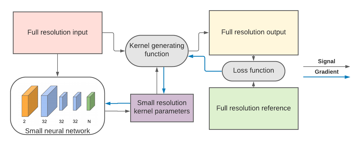
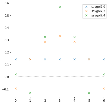
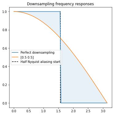
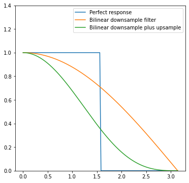
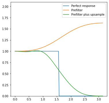
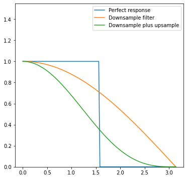
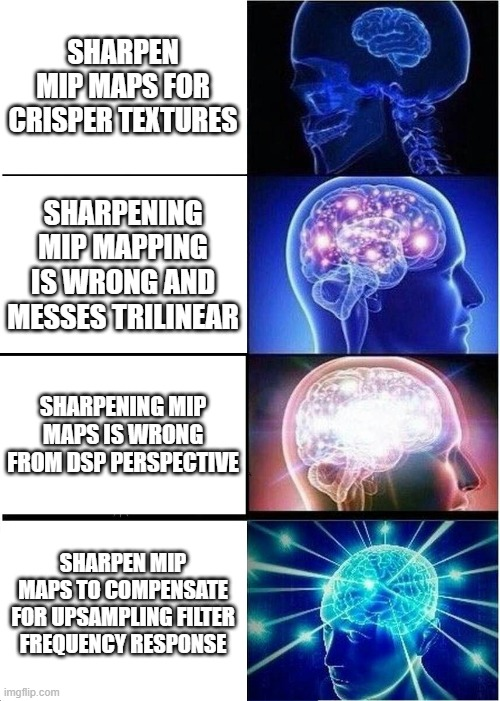
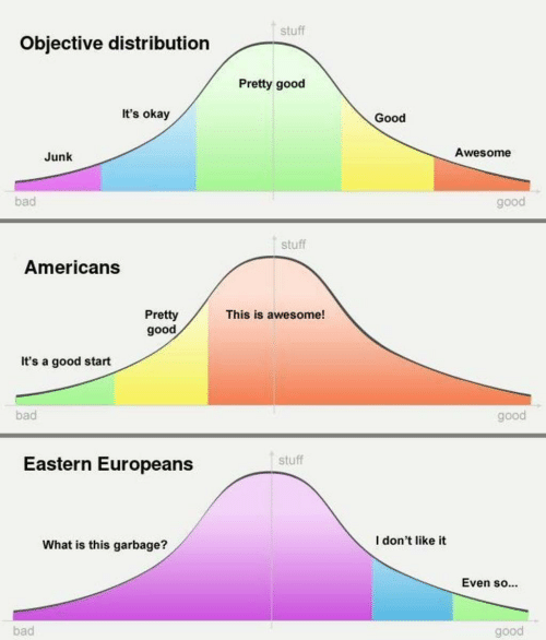
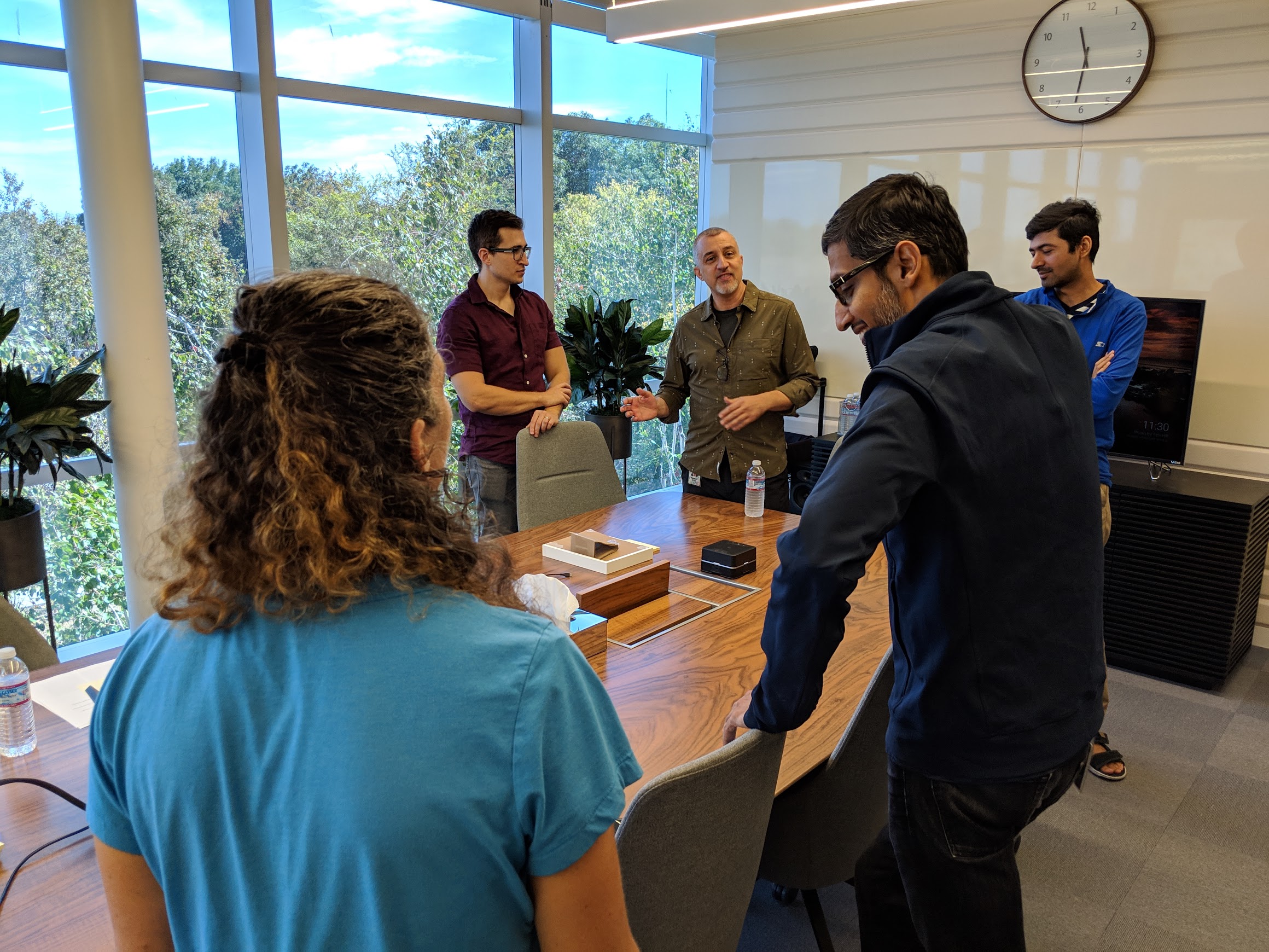
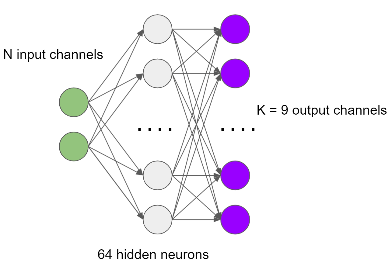
With infinite or large SNR, this goes towards direct inverse. With tiny SNR, we get cancellation of the inverse and asymptotically go towards zero. How does it look in terms of the frequency response?

Wiener shrinkage / regularization of the deconvolution – frequency response.

Notice how the inverse response is the same at the beginning of the curve with and without the regularization, but changes dramatically as the convolution attenuates more and more the highest frequencies. It goes to just zero at the Nyquist frequency – as we don’t have any information left there and it not just doesn’t amplify, but also removes noisy signal there. This can be thought of as actual combined deconvolution and denoising!

Here are two examples of the different noise levels and different deconvolution results:

**Left:** Original image. **Center:** Blurred through convolution. **Right:** Regularized deconvolution of a blurry and noisy image.
**Top**: Less noise. **Bottom**: More noise.

Worth noting how deconvolved results are still noisy, and still not perfectly reconstructing the original image – Wiener deconvolution can give optimal results in the least squares sense (though we simplified it as compared to original Wiener deconvolution and don’t take signal strength into account), but it doesn’t mean it will be optimal perceptually – it doesn’t “understand” our concepts of noise or blur. And it doesn’t adapt in any way to structures present in data…

Deconvolution in practice

We went through the theory of deconvolution, as well as some practical caveats like regularization against noise, so it’s time to put this into practice. I will start with a more “traditional”, slower method, followed by a simplified one, designed for real time and/or GPU applications.

Deconvolution by filter design

The first way of deconvolving is as easy as it gets; use a signal processing package to optimize a linear-phase FIR filter for the desired response. Writing your own that is optimal in the least-squares sense is maybe a dozen lines of Python code – later in the post we will use for a similar purpose. For this section, I used the excellent scipy.signal package.

convolution_filter = [0.25,0.5,0.25]
freq, response_to_invert = scipy.signal.freqz(convolution_filter)
noise_reg = 0.01
coeffs = 21
deconv_filter = scipy.signal.firls(coeffs , freq/np.pi, np.abs(response_to_invert)/(np.abs(response_to_invert)**2+(noise_reg)**2))

The earlier figures I generated this way:

If you’re curious, those are the plots of the generated filters:

Filter weights for two of our result deconvolution filters.

They should match the intuition – a more regularized filter can be significantly smaller in spatial support (doesn’t require “infinite” sampling to reconstruct frequencies closer to Nyquist), and it has less strong gains and less negative weights, preventing oversharpening of the noise. For the stronger filter, we are clearly utilizing all the samples, and most likely a larger filter would work better. Here is a comparison of desired vs actual frequency responses:

Frequency responses of two of our result deconvolution filters.

From here, one can go deeper into signal processing theory and practice of filter design – there are different filter design methods, different trade-offs, different results.

But I’d like to offer an alternative method that has a larger error, but is much better suited for real time applications.

Deconvolution by simple filter combination

Finding direct deconvolution filters through filter design works well, but it has one big disadvantage – resulting filters are huge, like 21 taps in the above example.

With separable filtering this might be generally ok – but if one was to implement a non-separable one, using 441 samples is prohibitive. Finding those 21 coefficients is also not instantaneous (require a pseudoinverse of a 21×21 matrix; or in case of non-separable filtering, solving a system involving a 441×441 matrix! Cost can be cut by half or quarter using symmetry of the problem, but it’s still not real-time instantaneous).

In computer graphics and image processing we tend to decompose images to pyramids for faster large spatial support processing. We can use this principle here.

A paper that highly inspired me a while ago was “Convolution Pyramids” – be sure to have a read. But this paper uses a complicated method with a non-linear optimization, which works great for their use-case, but here would be an overkill.

For a simple application like deconvolution, we can use simply a sum of Laplacians resulting from Gaussian filtering instead.

Imagine that we have a bunch of Gaussian filters with sigmas 0.3, 0.6, 0.9, 1.2, 1.5 (chosen arbitrarily) and their Laplacians (difference between levels) plus a “unity” filter that we will keep at 1.0. This way, we have 4 frequency responses to operate with and to try adding to reach the target response:

Different Laplacian levels frequency responses.

In numpy, this would be something like this:

def gauss_small_sigma(x: np.ndarray, sigma: float):
  p1 = scipy.special.erf((x-0.5)/sigma*np.sqrt(0.5))
  p2 = scipy.special.erf((x+0.5)/sigma*np.sqrt(0.5))
  f = (p2-p1)/2.0
  return f / np.sum(f)

filters = [gauss_small_sigma(np.arange(-5, 5, 1), s) for s in (0.00001, 0.3, 0.6, 0.9, 1.2, 1.5)]
filters_laps = [np.abs(scipy.signal.freqz(a - b)[1]) for a,b in zip(filters[1:], filters)]
stacked_laps = np.transpose(np.stack(filters_laps))
target_resp = stacked_laps, target - np.ones_like(target)
regularize_lambda = 0.001
solution_coeffs = np.linalg.lstsq(stacked_laps.T.dot(stacked_laps) + regularize_lambda * np.eye(stacked_laps.shape[1]),
                                  stacked_laps.T.dot(target_resp))[0]

Here, solved coefficients are [-17.413, 54.656, -52.741, 20.025] and the resulting fit is very good:

Edit: just right after publishing I realized I missed one Laplacian from plots and the next figure. Off by one error – sorry about that. Hopefully it doesn’t confuse the reader too much.

We can then convert the Laplacian coefficients to Gaussian coefficients if we want. But it’s also interesting to see how contributing Laplacians look like:

Source blurry image, different enhanced Laplacians, and the resulting deconvolved image.

As before, the results are not great because we have a relatively large blur and some noise. To improve it for such a combination, we would need to look at some non-linear methods. It’s also interesting that Laplacians seem to be huge in range and value (with my visualization clipping!), but their contributions mostly cancel each other out.

Note that this least squares solve requires operating only on a 5×5 matrix, so it’s super efficient to solve every frame (possibly even per pixel, but I don’t recommend that). It also uses separable, easily optimizable filters.

I chose used blurs arbitrarily, to get some coverage of small sigmas (which can be implemented efficiently). My ex-colleagues had a very interesting piece of work and paper that shows that by iterating the original blur kernel (which can be done efficiently in the case of small blurs; but you pay the extra memory cost for storing the intermediates), you can get a closed form expression coming from a truncated Neumann series. I recommend checking out their work, while I propose a more efficient alternative for small blurs.

Even simpler filter for small blurs

The final trick will come from a practical project that I worked on, and where blurs we were dealing with were smaller in magnitude (sigmas of like 0.3-0.6). We also had a sharpening part of the pipeline with some interesting properties that was authored by my colleague Dillon. I will not dive here into the details of that pipeline.

The thing that I looked at was the use of the kernel used to generate Laplacians – which was extremely efficient on the CPU and DSP and used “famous” dilated a-trous filter. I recommend an older paper that explains well the signal processing “magic” of a repeated comb filtering. Its application for denoising can leave characteristic repeated artifacts due to non-linear blurring, but it’s excellent for generating non-decimating wavelets or Laplacians.

Here is a diagram that +/- explains how it works if you don’t have time to read the referenced paper:

Different comb filters and how combining them forms a form of non-decimating Laplacian pyramid or a non-decimating wavelet pyramid.

Notice how each next comb filter combined with the previous one approximates full lowpass filter better and better. To get even better results, one would need a better lowpass filter with more than 3 (or 9 in 2D) taps. Those 3 comb filters form also 3 Laplacians (unity vs Comb1, Comb 1 vs combined Comb 1 and 2, combined Comb 2 and 3 vs combined Comb 1 and 2).

I looked at using those to approximate small sigma deconvolution and for those small sigmas they fit perfectly:

How well does it work in practice on images? Very well!

**Top row**: Source image, blurred image with a small sigma, deconvolved image.
**Bottom row**: Contributing Laplacian enhancements.

This is for a larger sigma of 0.7. Note also the third coefficient is always close to 0.0, so we can actually use only 2 comb filters and have just 2 Laplacians.

This can be implemented extremely efficiently (two passes of 9 taps; or 4 passes of 3 taps!), requires inverting just a 2×2 matrix (closed formula) and this one could be done per pixel in a shader. My colleague Pascal suggested solving this over a quadrature instead of uniformly sampling the frequency response and even the Gramm matrix accumulation can be accelerated by an order or two of magnitude with not much loss of the fit fidelity.

Bonus – convolution in relationship to sharpening

As a small bonus, an extreme case – how well can a silly and simple unsharp mask (yes, that thing where you just subtract a blurred version of the image and multiply it and add back) approximate deconvolution..?

Using unsharp masking for deconvolution / deblurring.

Using unsharp masking for deconvolution / deblurring.
**Left:** Original image. **Center:** Blurred through convolution. **Right:** Unsharp mask deconvolution of a blurry and noisy image

There’s definitely some oversharpening and “fat edges”, but given an arbitrary, relatively large kernel and just a single operation it’s not too bad! For smaller sigmas it works even better. “Sharpening” is a reasonable approximation of mild deconvolution. I am always amazed how well some artists’ and photographers’ tricks work and have a relationship to more “principled” approaches.

Limitations of linear deconvolution and conclusions

My post described the most rudimentary basis of single image deconvolution – its theory, algebraic and frequency domain take on the problem, practical problems, and how to create filters for linear deconvolution.

The quality of linear filters deconvolving noisy signals is not great – still pretty noisy, while leaving images blurry. To address this, one needs to involve non-linearity – local data dependence in the deconvolution process.

Historically many algorithms used optimization / iteration combined with priors. One of the simplest and oldest algorithms worth checking out is Richardson-Lucy deconvolution (pretty good intro and derivation, matlab results), though I would definitely not use it in practice.

Large chunk of work in the 90s and 00s used iterative optimization with image space priors like total variation prior or sparsity prior. Those took minutes to process, produced characteristic flat textures, but also super clean and sharp edges and improved text legibility a lot – and not surprisingly, were used in forensics and scientific or medical imaging. And as always, multi-frame methods that have significantly more information captured over time worked even better – see this work from one of my ex-colleagues, which was later used in commercial video editing products.

Modern way to approach it in a single-frame (but also increasingly more for videos) setting is unsurprisingly through neural networks which are both faster, as well as give higher quality results than optimization based methods.

In my recent tech report I proposed to combine super small and cheap neural networks with “traditional” methods (NN operates at lower resolution and predicts kernel parameters for a non-ML algorithm) and got some decent results:

**Left:** Source image. **Middle:** Blurry and noisy image. **Right:** Deconvolution + denoising using a mix of a tiny neural network and a set of traditional kernels. While the noise is much stronger than in the examples above, we don’t see catastrophic magnification and wrong textures.

Any decent nonlinear deconvolution would detect and adapt to local features like edges or textures, and treat them differently from flat areas, trying to amplify blurred local structure, while ignoring the noise. This is a very fun topic, especially when reading about combinations of deconvolution and denoising, very often encountered in scientific and medical imaging, where one physically cannot acquire better data due to physical limitations, costs, or for example to avoid exposing patients to radiation or inconvenience.

Hope you enjoyed my post, it inspired you to look more at the area of deconvolution, and that it demystified some of the “deblurring”, “sharpening”, and “super-resolution” circle of confusion. 🙂

Posted in Code / Graphics | 5 Comments

Transforming “noise” and random variables through non-linearities

Posted on March 16, 2022 by bartwronski

This post covers a topic slightly different from my usual ones and something I haven’t written much about before – applied elements of probability theory.

We will discuss what happens with “noise” – a random variable – when we apply some linear and nonlinear functions to it.

This is something I encountered a few times at work and over time built some better understanding of the topic, learned about some different, sometimes niche methods, and wanted to share it – as it’s definitely not very widely discussed.

I will mostly focus on univariate case – due to much easier visualization and intuition building, but also mention extensions to multivariate cases (all presented methods work for multidimensional random variables with correlation).

Let’s jump in!

Motivation – image processing vs graphics

The main motivation for noise modeling in computational photography and image processing is understanding the noise present in images to either remove, or at least not amplify it during downstream processing.

Denoisers that “understand” the amount of noise present around each pixel can do a much better job (it is significantly easier) than the ones that don’t. So-called “blind denoising” methods that don’t know the amount of noise present in the image actually often start with estimating noise. Non-blind denoisers use the statistical properties of expected noise to help delineate it from the signal. Note that this includes both “traditional” denoisers (like bilateral, NLM, wavelet shrinkage, or collaborative filtering), as well as machine learning ones – typically noise magnitude is provided as one of the channels.

Outside of denoising, you might need to understand the amounts of noise present – and noise characteristics – for other tasks, like sharpening or deconvolution – to avoid increasing the magnitude of noise and producing unusable images. There are statistical models like Wiener deconvolution that rely precisely on that information and then can produce provably optimal results.

Over the last few decades, there were numerous publications on modeling or estimating noise in natural images – and we know how to model all the physical processes that cause noise in film or digital photography. I won’t go into them – but a fascinating one is Poisson noise – uncertainty that comes from just counting photons! So even if we had a perfect physical light measurement device, just the quantum nature of light means we would still see noisy images.

This is how most people think of noise – noisy images.

In computer graphics, noise can mean many things. One that I’m not going to cover is noise as a source of structured randomness – like Perlin or Simplex noise. This is a fascinating topic, but doesn’t relate much to my post.

Another one is noise that comes from Monte Carlo integration with a limited number of samples. This is much more related to the noise in image processing, and we often want to denoise it with specialized denoisers. Both fields even use the same terminology from probability theory – like expected value (mean), MSE, MAP, variance, variance-bias tradeoff etc. Anything I am going to describe relates to it at least somewhat. On the other hand, the main difficulty with modeling and analyzing rendering Monte Carlo noise is that it is not just additive white Gaussian, and depends a lot on both integration techniques, as well as even just the integrated underlying signal.

Monte Carlo noise in rendering – often associated with raytracing, but any stochastic estimation will produce noise.

The third application that is also relevant is using noise for dithering. I had a series of posts on this topic – but the overall idea is to prevent some bias that can come from quantization of signals (like just saving results of computations to a texture) by adding some noise. This noise will be transformed later just like any other noise (and the typical choice of triangular dithering distribution makes it easier to analyze using just statistical moments). This is important, as if you perform for example gamma correction on a dithered image, the distribution of noise will be uneven and – furthermore – biased! We will have a look at this shortly after some introduction.

Dithering noise can be used to break up bad looking “banding”. Both left and right images use only 8 values!

Noise and random variables

My posts are never rich with formalism or notation and neither will this one be, but for this math-heavy topic we need some preliminaries.

When discussing “noise” here, we are talking about some random variable. So our “measurement” or final signal is whatever the “real” value was plus some random variable. This random variable can be characterized by different properties like the underlying distribution, or properties of this distribution – mean (average value), variance (squared standard deviation), and generally statistical moments.

After than the mean (expected value), the most important statistical moment is variance – squared standard deviation. The reason we like to operate on variance instead of directly standard deviation is that it is additive and variance scaling laws are much simpler (I will recap them in the next section).

For example in both multi-frame photography and Monte Carlo, variance generally scales down linearly with the sample count (at least when using white noise) – which means that the standard deviation will scale down with familiar “square root” law (to get reduction of noise standard deviation by 2, we need to take 4x more samples; or to reduce it by 10, we need 100 samples).

We will use a common notation:

Capital letters X, Y, Z will denote random variables.

Expected value (mean) of a random variable will be E(X).

Variance of a random variable will be var(X), covariance of two variables cov(X, Y).

Alternatively, if we use a vector notation for multivariate random variables and assume X is a random vector, covariance of the two is going to be just cov(X).

Letters like a, b, c, or A, B, C will denote either scalar or matrix linear transformations.

Linear transformations

To warm up, let’s start with the simplest and most intuitive case – a linear transformation of noise / a random variable. If you don’t need a refresher, feel free to skip to the “Including nonlinearities” section.
If we add some value to a random variable X, the mean E(X + a) is going to be simply E(X) + a.

The standard deviation or variance is not going to change – var(X + a) == var(X). This follows both intuition (simply “shifting” a variable), and should be obvious from the mathematical definition of variance as the second central moment – E((Y – E(Y))^2) – we remove the shared offset.

Things get more interesting – but still simple and intuitive – once we consider a scaling transformation.

E(aX) is a * E(X), while var(a * X) == a^2 * var(X). Or, generalizing to covariances, cov(a * X, b * Y) == a * b * cov(X, Y).

Why squared? In this case, I think it is simpler to think about it in terms of standard deviation. We expect the standard deviation to scale linearly with variable scaling (“average distance” will scale linearly), and variance is standard deviation squared.

When adding two random variables, the expected values also add. What is less intuitive is how the variance and standard deviation behave when adding two random variables. Bienaymé’s identity tells us that:

var(X + Y) == var(X) + var(Y) + 2*cov(X, Y).

In case of uncorrelated random variables, it is simply the sum of those variables – but it’s a common mistake if you use the variance sum formula and don’t check for variable independence! This mistake can happen quite commonly in image processing – when you introduce correlations between pixels through operations like blurring, or more generally – convolution.

Interesting aspect of this is when the covariance is negative – then we will observe less variance of the sum of the two variables as compared to just the sum of their variances! This is useful in practice if we introduce some anti-correlation on purpose – think of… blue noise. When averaging anti-correlated noise values, we will observe that the variance goes down faster than simple square root scaling! (This might not be the case asymptotically, but definitely happens at low sample counts and this is why blue noise is so attractive for real-time rendering)

Here is an example of a point set that is negatively correlated – and we can see that if we compute x + y (project on the shown line), the standard deviation on this axis will be lower than on original either x or y:

Putting those together

Let’s put the above identities to action in two simple cases.

The first one is going to be calculation of mean and variance of average of two variables. We can note (X + Y) / 2 as X / 2 + Y / 2. We can see that the E((X + Y) / 2) will be just (E(X) + E(Y)) / 2, but the variance is var(X)/4 + var(Y)/4 + cov(X, Y)/2.

If var(X) == var(Y) and cov(X, Y) == 0, we get the familiar formula of var(X) / 2 – linear variance scaling.

The second one is a formula of transforming covariances. If we apply a transformation matrix A to our variance/covariance matrix, it becomes A cov(X) A^T. I won’t derive it, but it is a direct application of all of the above formulas and re-writing it in a linear algebra form. What I like about it is the neat geometric interpretation – and relationship to the Gram matrix. I have looked at some of it in my post about image gradients.

Expressing covariance in matrix form is super useful in many fields – from image processing to robotics (Kalman filter!)

**Left:** Two independent random variables, covariance matrix [[1, 0], [0, 9]]. **Right:** after rotation, our new two variables are correlated, with covariance matrix [[10, 10], [10, 10]].

Typical noise assumptions

With some definitions and simple linear behaviors clarified, it’s worth to quickly discuss what kind of noise / random variable we’re going to be looking at in computer graphics or image processing. Most denoisers assume AWGN – additive, white, Gaussian noise.

Let’s take it piece by piece:

Additive – means that noise is added to the original signal (and not for example multiplied),
White – means that every pixel gets “corrupted” independently and there are no spatial correlations,
Gaussian – assumption of normal (Gaussian) distribution of noise on each pixel.

Why is this a good assumption? In practice, Poisson noise from counting photons can reasonably resemble an additive Gaussian distribution – and we count every pixel separately.

The same is not true for electrical measurement noises – there are many non-Gaussian components, there are some mild spatial noise correlations resulting from shared electric readout circuitry – and while some publications go extensively into analyzing it, assumption of white Gaussian is “ok” for all but extremely low light photography use-cases. When adding or averaging a lot of different noisy components (and there are many in electric circuitry), the sum eventually gets close enough to Gaussian due to the Central Limit Theorem.

For dithering noise, we typically inject this noise ourselves – and know if it’s white, blue, or not noise at all (patterns like Bayer). Similarly we know if we’re dealing with uniform, or (preferred) triangular distribution – which is not Gaussian, but gets “close enough” for similar analysis.

When analyzing noise from Monte Carlo integration, all bets are off. This noise is definitely not Gaussian, depending on the sampling scheme, sampled functions, most often non white, and generally “weird”. One advantage Monte Carlo denoisers have is strong priors and the use of auxiliary buffers like albedo or depth to guide the denoising – which provides such a powerful additional signal that it usually compensates for the noise characteristics “weirdness”. Note however that if we were to measure its empirical variance, all methods and transformations described here would work the same way.

In all of the uses described above, we initially assume that the noise is zero-mean – expected value of 0. If it wasn’t, it would be considered as the bias of the measurement. All the above linear transformations (adding zero mean noises, multiplying zero mean etc) preserve it. However, we will see now how even zero mean noise can result in non-zero mean and bias after other common transformations.

Including nonlinearities – surprising (or not?) behavior

Let’s start with a quiz, how would you compare the brightness of the three images below:

Central image is clean, the left one has noise added in linear space, the right one in gamma space – noise magnitude is small (as compared to signal) and the same between two images.

This is not a tricky human vision system question – at least I hope I’m not getting into some perceptual effects where display and surround variables twist the results – but I see the image on the left as significantly darker in the shadows as compared to the other two ones – which are hard to compare, as in some areas one seems brighter than the other one.

To emphasize this has nothing to do with perception, when computing the numerical average of all three images, it is different as well: 0.558, 0.568, 0.567. The left one is the darkest indeed.

This is something that surprised me a lot the first time I encountered it and internalized it – the choice of your denoising or blurring color / gamma space will affect the real average brightness of the image! This goes the same for other operations like sharpening, convolution etc.

If you denoise, or even blur an image (reducing noise) in linear space, it will be brighter than if you blurred it in gamma space.

Let’s have a look at why that is. Here is a synthetic test – we assume a signal of 0.2 and the same added zero mean noise, one in linear, one in gamma space (sqrt of the signal which was squared before; with a linear ramp below 0 to avoid a sqrt of negative numbers):

Black line marks the measured, empirical mean, and read line marks mean +/- standard deviation. Adding zero mean noise and applying a non-linearity changes the mean of the signal!

It also changes the standard deviation (much higher!) and skews and deforms the distribution – definitely not a Gaussian anymore.

To start building an intuition, think of a bimodal, discrete noise distribution – one that produces values of either -0.04, or 0.04. Now if we add it to a signal of 0.04 and remap with a sqrt nonlinearity, one value will be sqrt(0.0) == 0, the other one sqrt(0.08) ~=0.283. Their average is ~0.14, significantly below 0.2 of the square root of the same image that would have no noise.

The nonlinearity is “pushing” points on either side further or closer from the original mean, changing it.

Let’s have a look at an even more obvious example – a quadratic function, squaring the noisy signal.

If we square zero mean noise, we obviously cannot expect it to remain zero mean. All negative values will become positive.

Mean change was something that truly surprised me the first time I saw it with the square root / gamma, but looking at the squaring example, it should be obvious that it’s going to happen with non-linear transformations.

Change of variance / standard deviation should be much more expected and intuitive, possibly also just the change of the overall distribution shape.

But I believe this mean change effect is ignored by most people who apply some non-linearities to noisy signals – for example when dithering and trying to compensate for the sRGB curve that would be potentially applied on writing to a 8bit buffer. If you dither a linear signal, but save to a sRGB texture – you will not only introduce varying noise depending on the pixel brightness (more in the shadows) and be unable to find optimal value – it will be either too small in highlights, or too large in the shadows, but also and even worse – shift the brightness of the image in the darkest regions!

We would like to understand the effects of non-linearities on noise, and in some cases to compensate for it – but to do it, first we need a way of analyzing what’s going on.

We will have a look at three different relatively simple methods to model (and potentially compensate for) this behavior.

Nonlinearity modeling method one – noise transformation Monte Carlo

The first method should be familiar to anyone in graphics – Monte Carlo and a stochastic estimation.

This method is very simple:

Draw N random samples that follow the input distribution,
Transform the samples with a nonlinearity,
Analyze the resulting distribution (empirical mean, variance, possibly higher order moments).

This is what we did manually with the two above examples. In practice, we would like to estimate the effect of non-linearity applied on a measured noisy signal with different signal means.

We could enumerate all possible means and standard deviations we are interested in – but in practice, dealing with continuous variables, enumerating all values is impossible – we’d need to create a look-up table – sample and tabulate standard deviation and signal mean ranges, compute empirical mean/standard deviation, and interpolate in between, hoping the sampling is dense enough that the interpolation works.

This approach can be summarized in pseudo-code:

For sampled signal mean m
  For sampled noise standard deviation d
    For sample s
      Generate sample according to s and d
      Apply non-linearity
      Accumulate sample / accumulate moments
    Compute desired statistics for (m, d)

This is the approach we used in our Handheld Multi-frame Super-resolution paper to analyze the effect of perceptual remapping on noise. In our case, due to the camera noise model (heteroscedastic Gaussian as an approximation of mixed Gaussian + Poisson noise) our mean and standard deviations were correlated, so we could end up with just a single 1D LUT. In robustness/rejection shader, we would look-up the pixel brightness value, and based on it read the expected noise (standard deviation and mean) from a LUT texture using hardware linear interpolation.

Normally you would want to use “good” sampling strategy – low discrepancy sequences, stratification etc. – but this is beyond the topic of this post. Instead, here is the simplest possible / naive implementation for the 1D case in Python:

def monte_carlo_mean_std(orig_mean: float,
                         orig_std: float,
                         fun : Callable[[np.ndarray], np.ndarray],
                         sample_count: int = 10000) -> Tuple[float, float]:
  samples = np.random.normal(size=sample_count) * orig_std + orig_mean
  transformed = fun(samples)
  return np.mean(transformed), np.std(transformed)

Let’s have a look at what happens with the two functions used before – first sqrt(max(0, x)):

The behavior around 0 is especially interesting:

We observe both an increase in standard deviation (more noise) as well as a significant mean shift. Our signal with mean originally starting at 0 after the transformation starts way above 0. The effect on mean minimizes once we go higher and curves converge, but the standard deviation decreases instead – we will have a look at why in a second.

But first, let’s have a look at the second function, squaring:

And zoomed in behavior around 0:

Here behavior around 0 isn’t particularly insightful – as we expected, mean increases, and the standard deviation is minimal. However when we look at the unzoomed plot, some curious behavior emerges – it looks like the plot of the standard deviation is +/- linear. Coincidence? Definitely not! And we’ll have a look at why – while describing the second method.

Nonlinearity modeling method two – Taylor expansion

When you can afford it (for example, you can pre-tabulate data, deal with only univariate / 1D case etc), Monte Carlo simulation is great. On the other hand, it suffers from the curse of dimensionality and can get very computationally expensive to get reliable answers. Sampling all possible means / standard deviations becomes impractical and prone to undersampling and being noisy / unreliable itself.

The second analysis method relies on the very common engineering and mathematical practice – when you need to know only “approximate” answers of certain “well behaved” functions – linearization, or more generally – Taylor series expansion.

The idea is simple – once you “zoom-in”, many common functions can resemble tiny straight lines (or tiny polynomials) – where the more you zoom-in on a continuous function, the closer it resembles a polynomial.

What happens if we treat the analyzed non-linear function as a locally linear or locally polynomial and use it to analyze the transformed moments from the direct statistical moment definitions? We end up with neat, analytical formulas of the new transformed statistical moment values!

Wikipedia has some of the derivations for the first two moments (mean and variance).

Relevant formulas for us – second order approximation of mean and the first of variance – are: and .

Let’s have a look at those and try to analyze them before using them.

The first observation is that the mean doesn’t change based on the first derivative of the function, only on the second one (plus obviously further terms). Why? Because the linear component is anti-symmetric around the mean – so the influences on both sides cancel out. This will be generally true for even/odd powers.

The second observation is that if we apply those formulas to the linear transformation a * x, we get the exact formulas – because the linear approximation perfectly “approximates” the linear function.

Variance scaling quadratically with the first derivative (plus error / further terms) is exactly what we expected! Also from this perspective, the above plots of the Monte Carlo of the quadratic function transformed statistical moments makes perfect sense (dx^2 / dx == 2x) – standard deviation will scale linearly with signal strength.

We could compute derivatives manually when we know them – and you probably should, writing for numerical stability, optimal code, and preventing any singularities. But you can also use the auto differentiating frameworks to write once and experiment with different functions. We can write the above as small Jax code snippet:

def taylor_mean_std(orig_mean: float,
                    orig_std: float,
                    fun : Callable[[jnp.ndarray], jnp.ndarray]) -> Tuple[float, float]:
  first_derivative = jax.grad(fun)(orig_mean)
  second_derivative = jax.grad(jax.grad(fun))(orig_mean)
  orig_var = orig_std * orig_std
  taylor_mean = fun(orig_mean) + orig_var * second_derivative / 2.0
  var_first_degree = orig_var * np.square(first_derivative)
  var_second_degree = -np.square(second_derivative) * orig_var * orig_var / 4.0
  taylor_var = var_first_degree + var_second_degree
  return taylor_mean, np.sqrt(np.maximum(taylor_var, 0.0))

And we get almost the same results as Monte Carlo:

This shouldn’t be a surprise – quadratic function is approximated perfectly by a 2nd degree polynomial, because it is a 2nd degree polynomial.

For such an “easy”, smooth, continuous use-cases with convergent Taylor series, this method is perfect – closed formula, very fast to evaluate, extends to multivariate distributions and covariances.

However, if we look at sqrt(max(0, x)) we will see in a second why it might not be the best method for other use-cases.

If you remember how derivatives of the square root look like (and that a piecewise function is not everywhere differentiable) you might predict what the problem is going to be, but let’s look first at how poor approximation it is as compared to Monte Carlo:

The approximation of mean is especially bad – going towards negative infinity.

d/dx(sqrt(x)) = 1/(2 sqrt(x)), and the second derivative d/dx((dsqrt(x))/(dx)) = -1/(4 x^(3/2)). Both will go towards infinity / negative infinity at 0 – and the square root is “locally vertical” around zero!

Basically, Taylor series is very poor at approximating the square root close to 0:

I generated the above plot also using Jax (it’s fun to explore the higher order approximations and see how they behave):

def taylor(a: float,
           x: jnp.ndarray,
           func: Callable[[jnp.ndarray], jnp.ndarray],
           order: int):
  acc = jnp.zeros_like(x)
  curr_d = func
  for i in range(order + 1):
    acc = acc + jnp.power(x - a, i) * curr_d(a)  / math.factorial(i)
    curr_d = jax.grad(curr_d)
  return acc

Going back to our sqrt – for example at 0.001, the first derivative of sqrt is 15.81. At 0.00001, it is 158.11.

With local linearization (pretending only 1st component of the Taylor series matters), this would mean that the noise standard deviation would get boosted by a factor of 158, or variance by 25000!

And the above ignores the effect of “clamping” below 0 -> with a standard deviation of 0.1 and signal means of comparable or smaller magnitudes, many original samples will be negative, and the square root Taylor series obviously doesn’t know anything about it and that we used a piecewise function.

Other than the quality of Taylor series approximation that can be poor for certain functions, to get reliable results we would need to make sure that the noise standard deviation is significantly smaller than the local derivative.

I’ll remark here on something seemingly unrelated. Did you even wonder why Rec. 709 OETF (the same with sRGB) has a linear segment?

This is to bound the first derivative! By limiting the maximum gain to 4.5, we also bound how much noise can get amplified and avoid nasty singularities (a derivative that goes towards infinity). This can matter quite a lot in many applications – and the effect on local noise amplitude is one of the factors.

Even simpler case where Taylor series approximation breaks is “rectified” noise remapping, simple max(x, 0):

Not surprisingly, with such a non-smooth, piecewise function, derivative above 0.0 (equal simply to 1.0) doesn’t tell us anything about the behavior below 0.0 and is unable to capture any of changes of mean and standard deviation…

Overall, Taylor expansion can work pretty well – but you need to be careful and check if it makes sense in the used context – is the function well approximated by a polynomial? Is the noise magnitude significantly smaller than the local standard deviation?

Nonlinearity modeling method three – Unscented transform

As the final “main” method, let’s have a look at something that I have heard of only a year ago from a coworker who mentioned this in passing. The motivation is simple and in a way graphics-related.

If you ever did any Monte Carlo in rendering, I am sure you have used importance sampling – a method of strategically drawing and weighting samples that resembles the analyzed function as close as possible to reduce the Monte Carlo error / variance.

Importance sampling is unbiased, but its most extreme, degenerate form sometimes used in graphics – most representative point (see Brian Karis’s notes and linked references) is biased – as it takes only a single sample and always the same. This is extreme – approximating the whole function with just one sample! One would expect it to be a very poor representation – but if you pick a “good” evaluation point, it can work pretty well.

In math and probability, there is a similar concept – unscented transform. The idea is simple – for N dimensions, pick N+1 sample points (extra degree of freedom needed to compute mean), transform them through non-linearity, and then compute the empirical mean and variance. Yes, that simple! It has some uses in robotics and steering systems (in combination with Kalman filter) and was empirically demonstrated to work better than linearization (Taylor series) for many problems.

Jeffrey Uhlman (author of the unscented transform) proposed a method of finding the sample points through a Cholesky decomposition of the covariance matrix, and for example in 2D those points are:

In 1D, points are two and trivial – mean +/- standard deviation.

Thus, the code to compute this transformation is also trivial:

def unscented_mean_std(orig_mean: float,
                       orig_std: float,
                       fun : Callable[[np.ndarray], np.ndarray]) -> Tuple[float, float]:
  first_point = fun(orig_mean - orig_std)
  second_point = fun(orig_mean + orig_std)
  mean = (first_point + second_point) / 2.0
  std = np.abs(second_point - first_point) / 2.0
  return mean, std

For the square function, results are almost identical to MC simulation (slightly deviating around 0):

For the challenging square root case, in large range it is pretty ok and close:

However if we zoom-in around 0, we see some differences (but no “exploding” effect):

I marked with the black line the original standard deviation – pretty interesting (but not surprising?) that this is where it starts to break – but always remaining stable.

The max(x, 0) case while not perfect – is also much closer:

Unscented transform is similar to biased, undersampled Monte-Carlo – it will miss behavior beyond +/- standard deviation, and also undersample between two evaluation points – but should work reasonably well for a wide variety of cases.

I will return to final recommendations in the post summary, but overall if you don’t have a huge computational budget and analyzed non-linear functions don’t behave well, I highly recommend this method.

Bonus nonlinearity modeling methods – analytical distributions

The final method is not a single method, but a general observation.

I am pretty sure most of my blog readers (you, dear audience 🙂 ) are not mathematicians and I’m not one either – even if we use a lot of math in our daily work and many of us love it. When you are not an expert of a domain (like probability theory), it’s very easy to miss solutions to already solved problems and try reinventing them.

Statistics and probability theory analyze a lot of distributions, and a lot of transformations of those distributions with closed formulas for mean, standard deviation and even further moments.

One example would be a rectified normal distribution and truncated normal distribution.

Those distributions can very easily arise in signal and image processing (if we miss information about negative numbers) – and there are existing formulas for their moments analyzed by mathematicians. One of my colleagues has successfully used it in extreme low light photography to remove some of the color shifts resulting from noise truncation during processing.

This is a general advice – it’s worth doing some literature search outside of your domain (can be challenging due to different terminology) and asking around – as it might have been a solved problem.

Practical recommendation and summary

In this post I have recapped effects of linear transformations of random variables, and described three different methods of estimating effects of non-linearities on the basic statistical moments – mean and variance/standard deviation.

This was a more theoretical and math heavy post than most of mine, but it is also very practical – all of those three methods were things I needed (and have successfully used) at work.

So… from all three, what would be my recommendation?

As I mentioned, I have used all of the above methods in shipping projects. The choice of particular one will be use-case dependent – what is your computational budget, how much you can precompute, and most importantly – how your non-linearities look like – the typical “it depends”.

If you can precompute, have the budget, and used functions are highly non-linear and “weird”? Use Monte Carlo! Your non-linear functions are almost polynomial and “well behaved”? Use the Taylor series linearization. A general problem and a tight computational budget? I would commonly recommend the unscented transform.

…I might come back to the topic of noise modeling in some later posts, as it’s both a very practical and very deep topic, but that’s it for today – I hope it was insightful in some way.

Posted in Code / Graphics | Tagged blue noise, graphics, graphics programming, image processing, jax, mathematics, maths, noise, programming, python | Leave a comment

Fast, GPU friendly, antialiasing downsampling filter

Posted on March 7, 2022 by bartwronski

In this shorter post, I will describe a 2X downsampling filter that I propose as a “safe default” for GPU image processing. It’s been an omission on my side that I have not proposed any specific filter despite writing so much about the topic and desired properties. 🙂

I originally didn’t plan to write this post, but I was surprised by the warm response and popularity of me posting a shadertoy with this filter.

I also got asked some questions about derivation, so this post will focus on it.

TLDR: I propose a 8 bilinear tap downsampling filter that is optimized for:

Good anti-aliasing properties,
Sharper preservation of mid-frequencies than bilinear,
Computational cost and performance – only 8 taps on the GPU.

I believe that given its properties, you should use this filter (or something similar) anytime you can afford 8 samples when downsampling images by 2x on a GPU.

This filter behaves way better than a bilinear one under motion, aliases less, is sharper, and is not that computationally heavy.

You can find the filter shadertoy here.

Here is a simple synthetic data gif comparison:

**Left:** Proposed 2x downsampling filter. **Right:** bilinear downsampling filter.

If for some reason you cannot open the shadertoy, here is a video recording:

Red: classic box/bilinear downsampling filter. Green: proposed filter. Notice how almost all aliasing is gone – except for some of diagonal edges.

Preliminaries

In this post, I will assume you are familiar with the goals of a downsampling filter.

I highly recommend at least skimming two posts of mine on this topic if you haven’t, or as a refresher:

Bilinear down/upsampling, aligning pixel grids, and that infamous GPU half pixel offset

Processing aware image filtering: compensating for the upsampling

I will assume we are using “GPU coordinates”, so a “half texel offset” and pixel grids aligned with pixel corners (and not centers) – which means that the described filter is going to be even-sized.

Derivation steps

Perfect 1D 8 tap filter

A “perfect” downsampling filter would preserve all frequencies below Nyquist with a perfectly flat, unity response, and remove all frequencies above Nyquist. Note that a perfect filter from the signal processing POV is both unrealistic, and potentially undesirable (ringing, infinite spatial support). There are different schools of designing lowpass filters (depending on the desired stop band or pass band, transition zone, ripple etc), but let’s start with a simple 1D filter that is optimal in the simple least squares sense as compared to a perfect downsampler.

How do we do that? We can either solve a linear least squares system of equations on the desired frequency response (from a sampled Discrete-Time Frequency Response of a filter), or do a gradient descent using a cost function. I did the latter due to its simplicity in Jax (see a post of mine for example optimizing separable filters or about blue noise dithering through optimization).

If we do this for 8 samples, we end up with a frequency response like this:

We can see that it is both almost always sharper than bilinear under Nyquist, as well as removes much less of the high frequencies. There is a “ripple” and some frequencies will be boosted / sharpened, but in general it’s ok for downsampling. Such ripples are problematic for continuous resampling filters – can cause some image frequencies to “explode”, but even creating 10 mip maps, we shouldn’t get any problems – as each levels “boost” will translate to different original frequencies, so they won’t accumulate.

Moving to 2D

Let’s take just an outer product of 1D downsampler and produce an initial 2D downsampler:

**Left:** Perfect downsampler frequency response. **Center:** Bilinear response. **Right:** Our initial 8×8 2D filter response.

It is pretty good (other than slight sharpening), but we wouldn’t want to use a 8×8, so 64 tap filter (it might be ok for “separable” downsampling, which is often a good idea on CPU or DSP, but not necessarily on the GPU).

So let’s have a look at the filter weights:

We can see that many corner weights have magnitudes close to 0.0. Here are all the weights with magnitude below 0.02:

Why 0.02? This is just an ad-hoc number, magnitude ~10x lower than the highest weights. But when setting such a threshold, we can remove half of the filter taps! There is another reason I have selected those samples – bilinear sampling optimization. But we will come back to it in a second.

So we can just get rid of those weights? If we zero them out and normalize the filter, we get the following response:

**Left:** Perfect downsampler response. **Center:** Initial 8×8 filter response. **Right:** 32-tap “cross” filter response – some weights of a 64 tap filter zeroed out.

Some of the overshoots have disappeared! This is nice. What is not great though, is that we started to let through a bit more frequencies on diagonals – which kind of makes sense given the removal of diagonal weights. We could address that a bit by including more samples, but this would increase the total filter cost to 12 bilinear taps instead of 8 – for a minor quality difference.

But can slightly improve / optimize this filter further. We can either directly do a least-squares solve to minimize the squared error compared to a perfect downsampler, or just do a gradient descent towards it (while keeping the zeroed coefficients zero). The difference is not huge, only a few percent of difference on least squares error, but there is no reason not to do it:

**Left:** Perfect downsampler response. **Center:** Initial 32-tap “cross” filter response – some weights of a 64 tap filter zeroed out. **Right:** Re-optimized 32 tap filter response.

Now time for the ultimate performance optimization trick (as 32 tap filter would be prohibitively expensive for the majority of applications).

Bilinear tap optimization

Let’s have a look at our filter:

What is very convenient about this filter is having groups of 2×2 pixels that have the same sign:

When we have a group of 2×2 pixels with the same sign, we can try to approximate them with a single bilinear tap! This is a super common “trick” in GPU image processing. In a way, anytime you take a single tap 2×2 box filter, you are using this “trick” – but it’s common to explicitly approximate e.g. Gaussians this way.

If we take a sample that is offset by dx, dy and has a weight w, we end up with effective weights:

(1-dx)*(1-dy)*w, dx*(1-dy)*w, (1-dx)*dy*w, dx*dy*w.

Given initial weights a, b, c, d, we can optimize our coefficients dx, dy, w to minimize the error. Why will there be an error? Because we have one less degree of freedom in the (dx, dy, w) as compared to the (a, b, c, d).

This is either a simple convex non-linear optimization, or… a low rank approximation! Yes, this is a cool and surprising connection – we are basically trying to make a separable, rank 1 matrix. 2×2 matrix is at most rank 2, so rank 1 approximation in many cases will be good. This is worth thinking about – which 2×2 matrices will be well approximated? Something like [[0.25, 0.25], [0.25, 0.25]] is expressed exactly with just a single bilinear tap, while [[1, 0], [0, 1]] will yield a pretty bad error.

Let’s just use a simple numpy non-linear optimize:

def maximize_4tap(f):
  def effective_c(x):
    dx, dy, w = np.clip(x[0], 0, 1), np.clip(x[1], 0, 1), x[2]
    return w * np.array([[(1-dx)*(1-dy), (1-dx)*dy], [dx*(1-dy), dx*dy]])    
  def loss(x):
    return np.sum(np.square(effective_c(x) - f))
  res = scipy.optimize.minimize(loss, [0.5, 0.5, np.sum(f)])
  print(f, effective_c(res['x']))
  return res['x']

Note that this method can work also when some of the weights are of differing sign – but the approximation will not be very good. Anyway, in the case of the described filter, the approximation is close to perfect. 🙂

We arrive at the final result:

    vec3 col = vec3(0.0);
    col += 0.37487566 * texture(iChannel0, uv + vec2(-0.75777,-0.75777)*invPixelSize).xyz;
    col += 0.37487566 * texture(iChannel0, uv + vec2(0.75777,-0.75777)*invPixelSize).xyz;
    col += 0.37487566 * texture(iChannel0, uv + vec2(0.75777,0.75777)*invPixelSize).xyz;
    col += 0.37487566 * texture(iChannel0, uv + vec2(-0.75777,0.75777)*invPixelSize).xyz;
    
    col += -0.12487566 * texture(iChannel0, uv + vec2(-2.907,0.0)*invPixelSize).xyz;
    col += -0.12487566 * texture(iChannel0, uv + vec2(2.907,0.0)*invPixelSize).xyz;
    col += -0.12487566 * texture(iChannel0, uv + vec2(0.0,-2.907)*invPixelSize).xyz;
    col += -0.12487566 * texture(iChannel0, uv + vec2(0.0,2.907)*invPixelSize).xyz;

Only 8 bilinear samples! Important note: I assume here that UV is centered between 4 high resolution pixels – this is the UV coordinate you would use for bilinear / box interpolation.

Conclusions

This was a short post – mostly describing some derivation steps. But from a practical point of view, I highly recommend the proposed filter as a drop-in replacement to things like creating image pyramids for image processing or post-processing effects.

This matters for low resolution processing (for saving performance), or when we want to create a Gaussian-like pyramid (though with Gaussian pyramids we very often use more heavily lowpass filters and don’t care as much about preserving exactly below Nyquist).

If you look at the stability of the proposed filter in motion, you can see it is purely superior to box downsample – and not sacrificing any sharpness.

Bonus – use on mip maps?

I got asked an interesting question on twitter – would I recommend this filter for mip-map creation?

The answer is – it depends. For sure it is better than a bilinear/box filter. If you create mip-maps on the fly / in runtime, like from procedural textures, then the answer is – probably yes. But counter-intuitively, a filter that does some more sharpening or even lets through some aliasing might be actually pretty good and desireable for mipmaps! I wrote how when we downsample images, we should be aware of how we’re going to use them – including upsample or bilinear sampling, and might want to change the frequency response to compensate for it. Mip-mapping is one of those cases where designing a slightly sharpening filter might be good – as we are going to bilinearly upsample the image for trilinear interpolation or display later.

Posted in Code / Graphics | Tagged filtering, graphics, graphics programming, image processing, jax, postprocessing, signal processing | 6 Comments

Exposure Fusion – local tonemapping for real-time rendering

Posted on February 28, 2022 by bartwronski

Local tonemapping in action. HDRI texture credit: Greg Zaal, CC0.

In this post I want to close the loop and come back to the topic I described ~6y ago!

Local tonemapping (I’ll refer to it as LTM) – a component I considered a missing piece in video games rendering, especially with physically-based pipelines and using real/physical sky/sun models.

Global tonemapping is not enough for casual photography (where we don’t control the lighting), and while games can “hack” things, I considered LTM an almost a must have tool that can be used in some cases.

I have described a simple hacked solution that I implemented for God of War, but I was never happy with it – it helped in some scenes, but pushing it caused all kinds of ugly halo artifacts:

Local tonemapping as used in God of War. Description here.

Later I remember discussions on twitter about using “bilateral grid” (really influential older work from my ex colleague Jiawen “Kevin” Chen) to prevent some halos, and last year Jasmin Patry gave an amazing presentation about tonemapping, color, and many other topics in “Ghost of Tsushima” that uses a mix of bilateral grid and Gaussian blurs. I’ll get back to it later.

What I didn’t know when I originally wrote my post was that a year later, I would join Google, and work with some of the best image processing scientists and engineers on HDR+ – computational photography pipeline that includes many components, but one of the key signature ones is local tonemapping – the magic behind “HDR+ look” that is praised by both the reviewers and users.

The LTM solution is a fairly advanced pipeline, the result of the labor and love of my colleague Ryan (you might know his early graphics work if you ever used Winamp!) with excellent engineering, ideas, and endless patience for tweaks and tunings – a true “secret sauce”.

But the original inspiration and the core skeleton is a fairly simple algorithm, “Exposure Fusion”, which can both deliver excellent results, as well as be implemented very easily – and I’m going to cover it and discuss its use for real time rendering.

This post comes with a web demo in Javascript and obviously with source code. To be honest it was an excuse for me to learn some Javascript and WebGL (might write some quick “getting started” post about my experience), but I’m happy how it turned out.

So, let’s jump in!

Some disclaimers

In this post I will be using a HDRI by Greg Zaal.

Throughout the post I will be using ACES global tonemapper – I know it has a bad reputation (especially per-channel fits) and you might want to use something different, but its three js implementation is pretty good and has some of the proper desaturation properties. Important to note – in this post I don’t assume anything about the used global tonemapper and its curves or shapes – most will work as long as they reduce dynamic range. So in a way, this technique is orthogonal to the global tonemapping look and treatment of colors and tones.

Finally, I know how many – including myself – hate the “toxic HDR” look that was popular in the early noughties – and while it is possible to achieve it with the described method, it doesn’t have to be – this is a matter of tuning parameters.

Note that if you ever use Lightroom or Adobe Camera Raw to open RAW files in Photoshop, you are using a local tonemapper! Simply their implementation is very good and has subtle, reasonable defaults.

Localized exposure, local tonemapping – recap of the problem

In my old post, I went quite deep into why one might want to use a localized exposure / localized tonemapping solution. I encourage you to read it if you haven’t, but I’ll quickly summarize the problem here as well.

This problem occurs in photography, but we can look at it from a graphics perspective.

We render a scene with a physically correct pipeline, using physical values for lighting, and have an HDR representation of the scene. To display it, you need to adjust exposure and tonemap it.

If your scene has a lot of dynamic range (simplest case – a day scene with harsh sunlight and parts of the scene in shadows), picking the right exposure is challenging.

If we pick a “medium” exposure, exposing for the midtones, we get something “reasonable”:

On the other hand, details in the sunlit areas are washed out and barely visible, and information in the shadows is completely dark and barely visible.

You might want to render a scene like this – high contrast can be a desired outcome with some artistic intent. In some other cases it might not be – and this is especially important in video games that are not just pure art, but visuals need to serve gameplay and interactive purposes – very often, you cannot have important detail not visible.

If we try to reduce the contrast, we can start seeing all the details, but everything looks washed out and ugly:

We want to keep the original, punchy look, but still be able to see all the relevant details. How can we do that?

Let’s get back to selecting the exposure – here are three different exposures:

None of them is perfect when it comes to representing all details in the scene, but each one of them produces a clear, pleasant look in a certain area.

I have marked it with a green circle area “properly exposed” regions – where we can see all the details. Locally, in those regions, those images look perfect for our intent – and we are going to produce a single image that combines all of those.

Alternative solutions

It’s worth mentioning how this problem can be solved in other ways.

My previous post described some solutions used in photography, filmography, and video games. Typically it involves either manually brightening/darkening some areas (famous Ansel Adams dodge/burn aspects of the zone system), but it can start much earlier, before taking the picture – by inserting artificial lights that reduce contrast of the scene, tarps, reflectors, diffusers.

In video games it is way easier to “fake” it, and break all physicality completely – from lights through materials to post fx – and while it’s an useful tool, it reduces the ease and potential of using physical consistency and ability to use references and real life models. Once you hack your sky lighting model, the sun or artificial lights at sunset will not look correctly…

Or you could brighten the character albedos – but then the character art director will be upset that their characters might be visible, but look too chalky and have no proper rim specular. (Yes, this is a real anecdote from my working experience. 🙂 )

In practice you want to do as much as you can for artistic purposes – fill lights and character lights are amazing tools for shaping and conveying the mood of the scene. You don’t want to waste those, their artistic expressive power, and performance budgets to “fight” with the tonemapper…

Blending exposures

So we have three exposures – and we’d want to blend them, deciding per region which exposure to take.

There are a few ways to go about it, let’s go through them and some of their problems.

Per-pixel blending

The simplest option is very simple indeed – just deciding per pixel how to blend the three exposures depending on how well exposed they are.

This doesn’t work very well:

Ok, I take it even further – this is super ugly!

Everything looks washed out and weirdly saturated. It resembles a lot of the “toxic HDR” look mixed with washed out low contrast.

The problem is that even a dark region might have some bright pixels – and if we bring them down instead of up, it reduces the contrast.

Gaussian blending

The second alternative is simple – blurring the pixel luminance (a lot!) before deciding on how to adjust the local exposure / which exposure to use.

This is the approach I have described in my previous post and what we used for the God of War. And it can work “ok”, but generates pretty bad halos:

Bright regions trying to bring the dark ones down will leak onto medium exposure and dark regions, darkening them further and vice versa – dark regions strong influence will leak onto the surroundings. On a still image it can look acceptable, but with a video game moving camera it is visible and distracting…

Bilateral blending

Given that we would like to prevent bleeding over edges, one might try to use some form of edge-preserving or edge-stopping filter like bilateral. And it’s not a bad idea, but comes with some problems – gradient reversals and edge ringing.

I will refer you here to the mentioned excellent Siggraph presentation by Jasmin Patry who has analyzed where those come from.

In his Desmos calculator he demos the problem on a simple 1D edge:

Source and credit: Desmos calculator by Jasmin Patry

His proposed solution to this problem (to blend bilateral with Gaussian) is great and offers a balance between halos and edge/gradient reversals and ringing that can occur with bilateral filters.

But we can do even better and reduce the problem further through Exposure Fusion. But before we do, let’s look first however at a reasonable (but also flawed) alternative.

Guided filter blending

A while ago, I wrote about the guided filter – how local linear models can be very useful and in some cases can work much better (and more efficiently!) than a joint bilateral filter.

I’ll refer you to the post – and we will be actually using it later for speeding up the processing, so might be worth refreshing.

If we try to use a guided filter to transfer exposure information from low resolution / blurry image with blended exposure to full resolution, we end up with a result like this:

It’s actually not too bad, but notice that it tends to blur out some edges and reduce the local contrast as compared to the exposure fusion technique we’re going to have a look at next:

Exposure fusion

“Exposure fusion” by Mertens et al attempts to solve blending multiple globally tonemapped exposures (can be “synthetic” in the case of rendering), but in a way that preserves detail, edges, and minimizes halos.

It starts with an observation that depending on the region of the image and presence of details, sometimes you want to have a wide blending radius, sometimes very sharp.

Anytime you have a sharp edge – you want your blending to happen over a small area to avoid a halo. Anytime you have a relatively flat region – you want blending to happen over a large area, smoothen and be imperceptible.

The way authors propose to achieve it is through blending different frequency information with a different radius.

This might be somewhat surprising and it’s hard to visualize, but let me attempt it. Here we change the exposure rapidly over a small horizontal line section:

Notice how the change is not perceivable on the top of the image, this could be a normal picture, while on the bottom it is very harsh. Why? Because on top, the high frequency change correlates with high frequency information and image content change, while on the bottom it is applied to the low frequency information.

The key insight here is that you want frequency of the change to correlate with the frequency content of the image.

On low frequency, flat regions, we are going to use a very wide blending radius. In areas with edges and textures, we are going to make it steeper and stop around them. Changes in brightness are hidden by the edges or alternatively, smoothened out over large edgeless regions!

Authors propose a simple approach: Construct Laplacian pyramids for each blended image – and blend those Laplacians. Laplacian blending radius is proportional to the Laplacian radius – and can be trivially constructed by creating a Gaussian pyramid of the weights.

Here is a figure from the paper that shows how simple (and brilliant) the idea is:

Image source and credit: “Exposure Fusion”, T.Mertens, J.Kautz, F.Van Reeth

I will describe later some GPU implementation details and parameters used how to make it behave well, but first let’s have a look at the results:

This looks really good! Contrasty, punchy look, details visible everywhere. Compared to the global tonemapping (apologies for GIF banding artifacts):

What I like about this picture is the lack of halos, lack of washout effect, proper local contrast, proper details, overall relatively subtle look. This might not be the look you’d want for that scene – obviously this is an artistic process – but it looks correct.

Algorithm details

I highly encourage you to read the paper, but here is a short description of all of the steps:

Create “synthetic exposures” by tonemapping your image with different exposure settings. In general the more – the better, but 3 are a pretty good starting choice, allowing for separate control of “shadows” and highlights.
Compute the “lightness” / “brightness” image from each synthetic exposure. Gamma-mapped luminance is an extremely crude and wrong approximation, but this is what I used in the demo to simplify it a lot.
Create a Laplacian pyramid of each lightness image up to some level – more about it later. This last level will be just Gaussian-blurred, low resolution version of the given exposure, all the other will be Laplacian – difference between two Gaussian levels.
Assign a per-pixel weight to each high resolution lightness image. Authors propose to use three metrics – contrast, saturation, and exposure – closeness to gray. In practice if you want to avoid some of the over-saturated, over-contrasty look, I recommend using just the exposure.
Create a Gaussian pyramid of the weights.
On some selected coarse level (like on the 5th or 6th mip-map), blend the coarsest Gaussian lightness mip-maps with the Gaussian weights.
Go towards the finer pyramid levels / resolution – and on each level, blend Laplacians using a given level Gaussian and add it to the accumulated result.
Transfer the lightness to the full target image and do the rest of your tonemapping and color grading shenanigans.

Voila! We have an image in which edges (Laplacians) are blended at different scales with different radii.

In practice, getting this algorithm to look very well in multiple conditions (it has some unintuitive behaviors) requires some tricks and some tuning – but in a nutshell it’s very simple!

Optional – local contrast boost

One interesting option that the algorithm gives us is to boost the local contrast. It can be done in a few ways, but one that is pretty subtle and I like is to include the Laplacian magnitudes when deciding on the blending weights. Our effective weight will be Gaussian of the per-pixel weights times the absolute value of the magnitude. Note that generally this again is done per scale – so each scale weight is picked separately.

Produced local contrast boost can be visually pleasing:

It actually reduces some of the “flat” look that every LTM operator can produce when pushed to the extreme.

If you are a Lightroom user, their “Clarity” slider has a very similar effect and while the algorithm is proprietary (most likely a variant of “Local Laplacian Filter”), the general mechanism of action is very similar as well!

Extreme settings

I will describe algorithm / implementation parameters in the next section, but I couldn’t resist producing some “extreme toxic HDR” look as well – mostly to show that the algorithm is capable of doing so (if this is your aesthetic preference – and for some cases like architecture visualization it seems to be…).

Not my look and definitely in artificial territories, but still, not too bad – there are some dark halos here and there, weird washouts, but the algorithm seems to perform reasonably well.

Parametrization

Here are some of the algorithm parameters and the way I parametrized it.

Exposure

This one is the most straightforward. Exposure describes preferred overall average and “midtone” scene brightness.

Here are three exposure levels (for comparison – top row is with LTM off and the bottom is on):

Shadows and highlights

Shadows and highlights in my proposed parametrization describe how much to darken or brighten the synthetic exposures as compared to the global/middle exposure value.

Here is the same image with the same exposure with left having the highest value of “shadows” (biggest exposure boost of the brightest image), center with both of them at 0, and the right with maximum “highlights”:

Those are extreme and not recommended values – but the concept of tuning separately shadows and highlights is very important for artistic control over the tonemapping. It is part of the image and the look, and should be decided with artistic intent and for the scene mood.

Coarsest mip level

The final two important parameters are the most counter-intuitive.

When we decide up to which level we’d want to construct the pyramids, we decide which frequencies will be blended together (anything at that mip level and above). Setting the mip level to 0 is equivalent to full per-pixel weights and blending. On the other hand, setting it to maximum blends each level as Laplacian.

The lower the coarsest level, the more dynamic range compression there is – but also more washed out, fake-HDR look.

Here are mip levels 0, 5, 9:

Thing to notice is the increasing amount of local contrast (see for example the floor, especially close to table leg). The leftmost picture lacks some local contrast and gets washed out, but has the most dynamic range compression.

This might not be very clear, so I recommend you play with it in the demo to build some intuition.

Exposure preference sigma

This is the final parameter – it describes how “strong” the weighting preference is based on closeness of the lightness to 0.5. It affects the overall strength of the effect – with zero providing almost no LTM (all exposure weights are the same!), and with extreme settings producing artifacts and overcompressed look (pixels getting contribution only from a single exposure with some discontinuities):

(Notice the artifacts on the rightmost image on the table and when highlights blend with the midtones)

I again recommend you play with it yourself to build some intuition.

Algorithm problems

Overall, I like the algorithm a lot and find it excellent and able to produce great results.

The biggest problem is its counterintuitive behavior that depends on the image frequency content. Images with strong edges will compress differently, with a different look than images with weak edges. Even the frequency of detail (like fine scale – foliage vs medium scale like textures) matters and will affect the look. This is a problem as a certain value of “shadows” will brighten actual shadows of scenes differently depending on their contents. This is where artist control and tuning come into play. While there are many sweet spots, getting them perfectly right for every scenario (like casual smartphone photography) requires a lot of work. Luckily in games and adjusting it per scene it can be much easier.

The second issue is that when pushed to the extreme, the algorithm will produce artifacts. One way to get around it is to increase the number of the synthetic exposures, but this increases the cost.

Note that both of those problems don’t occur if you use it in a more “subtle” way, as a tool and in combination with other tools of the trade.

Finally, the algorithm is designed for blending LDR exposures and producing an LDR image. I think it should work with HDR pipelines as well, but some modifications might be needed.

GPU implementation

The algorithm is very straightforward to implement on the GPU. See my 300loc implementation, where those 300 lines include GUI, loading etc!

All synthetic exposures can be packed together in a single texture. One doesn’t need to create Laplacian pyramids and allocate memory for them – they can be constructed as a difference between Gaussian pyramids mip-maps. Creation of pyramids can be as simple as creating mips, or as complicated and fast as using compute shaders to produce multiple levels in one pass.

Note: I used the most simple bilinear downsampling and upsampling, which comes with some problems and would alias and flicked under motion. It also can produce diamond-shaped artifacts (an old post of mine explains those). In practice, I would suggest using a much better downsampling filter, and adjusting it for the upsampling operator. But for subtle settings this might not be necessary.

The biggest cost is in tonemapping the synthetic exposures (as expensive as your global tonemapping operator) – but one could use a simplified “proxy” operator – we care only about the correlation with the final lightness here.

Other than this, every level is just a little bit of ALU and 3 texture fetches from very low resolution textures!

How fast is it? I don’t have a way to profile it now (coding on my laptop), but I believe that if implemented correctly, it should definitely be under 1ms on even previous generation consoles.

But… we can make it even faster and make most computations happen in low resolution!

Guided upsampling

While it is doable (and possibly not too expensive) to compute the exposure fusion in full resolution, why not just compute it at lower resolution and transfer the information to the full resolution with a joint bilateral or a guided filter?

As long as we don’t filter out too much of the local contrast (in low resolution representation, sharp edges and details are missing), the results can be excellent. This idea was used in many Google research projects/products: HDRNet, Portrait mode, and for the tonemapping (it was again a fairly complex and sophisticated variation of this simple algorithm, designed and implemented by my colleague Dillon Sharlet).

I’ll refer you to my guided filter post for the details, but so far every single result that I have shown in this post was produced in ¼ x ¼ resolution and guided upsampled!

Here is a comparison of the computation at full, half, and quarter resolution, as a gif, as differences are impossible to see side-by-side:

Animated GIF showing results computed at full, half, and quarter resolution. Differences are subtle, and mostly on the floor texture.

I also had to crop as otherwise the difference was not noticeable – you can see it on the ground texture (high frequency dots) as well as a subtle smudge artifact on the chair back.

I encourage you to play with it in the demo app – you can adjust the “display_mip” parameter.

Summary

To conclude, in this post I came back to the topic of localized tonemapping, its general ideas and have described the “exposure fusion” algorithm with a simple, GPU friendly implementation – suitable for a simple WebGL demo (I release it to public domain, feel free to use or modify as much of it as you want).

It feels good to close the loop after 6y and knowing much more on the topic. 🙂

And a personal perspective – after those years, I am now even more convinced that having some LTM is a must as it’s an extremely invaluable tool. I hope this post convinced you so, and inspired you to experiment with it, and maybe implement it in your engine/game.

Posted in Code / Graphics | Tagged bilateral, graphics, graphics programming, image processing, postprocessing, tonemapping | Leave a comment

Light transport matrices, SVD, spectral analysis, and matrix completion

Posted on February 15, 2022 by bartwronski

Singular components of a light transport matrix – for an explanation of what’s going on – keep on reading!

In this post I’ll describe a small hike into the landscape of using linear algebra methods for analyzing seemingly non-algebraic problems, like light transport.

This is very common in some domains of computer science / electrical engineering (seeing everything as vectors / matrices / tensors), while in some others – like computer graphics – more occasional.

Light transport matrices used to be pretty common in computer graphics (for example in radiosity or more broadly, precomputed radiance transfer methods), so if some things in my post seem like rediscovering radiosity methods – they are; and I’ll try to mark the connections.

The first half of the post is very introductory and re-explaining some of the common light transport matrix concepts – while the second half will cover some more interesting and advanced, open ideas / problems around singular value decomposition and spectral analysis of those light transport matrices.

I’ll mention two ideas I had that seemed novel and potentially useful – and spoiler alert – one was not novel (I found prior work that describes exactly the same idea), and the other one is interesting and novel, but probably not very practical.

(While in academia there is no reward for being second to do something, in real life there is a lot of value in the discovery journey you made and idea seeds planted in your head. 🙂 )

And… it’s an excuse to produce some cool, educational figures and visualizations, plus connect some seemingly unconnected domains, so let’s go.

What is light transport and light transport matrix?

Light transport is in very broad, handwavy terms the physical process of light traveling from destination A to destination B and potentially interacting with the environment along the way. Light transport is affected by the presence of occlusions, participating media, angles at which surfaces are to each other, materials that emit or absorb certain amounts of light.

One can say that the goal of rendering is to compute the light transport from the scene to the camera – which is as broad as it gets, this is like almost all computer graphics!

We will simplify and heavily constrain this to a toy problem in a second.

Light transport matrices

Before describing the simplifications we will make, let’s have a look at how light transport could be represented in an extremely simple scene that consists of three, infinitesimal (infinitely small) points A, B, C. Infinitesimal / differential elements are very common in light transport – we assume they have a surface, we compute light transport on this surface, but this surface goes asymptotically towards 0, so we can ignore integrating over this surface.

If we “somehow” compute how much light gets emitted from the point A to point B and C, from point B to A and C, and C to A and B, we can represent it in a 3×3 matrix:

A few things to note here: in this case, we look only at a single bounce of light – therefore values on the diagonal are zero – shining some light on point A doesn’t transmit any light to itself through any other paths.

In this case, the presented matrix is symmetric – we assume the same amount of light gets transmitted from A to B and from B to A.

This doesn’t need to be the case – there can definitely be some non symmetric matrices present, though many of their “components” and elements that contribute to their values are symmetric.

If point A has no direct path to point B, point B also won’t have a path to point A.

Thus a visibility or shadowing term of a direct light transport matrix would be similar.

The same goes for so-called form factor (or view factor).

I will not go too much into the form factor matrix, but it is interesting that assuming full, perfect discretization and coverage of the scene it is not only strictly positive, symmetrical, but also double stochastic matrix – all rows and columns sum to 1.0.

We have a light transport matrix… Why is it useful? It allows us to express interesting physical interactions by simple mathematical operations! One example (more on that later) is that by computing M + M @ M – a matrix addition and multiplication – one can express computation of two bounces of light in the scene.

We can also compute the lighting in the scene when we treat point A as emitting some light.

Assuming that we put there 1.0, we end with a simple matrix – vector multiplication like:

So with a single algebraic operation, we computed light received at all points of the scene after two bounces of GI lighting.

Assumptions and simplifications

Let’s make the problem easy to explain and play with by doing some very heavy simplifications and assumptions I’ll be using throughout the post:

I will assume that we are looking only at a single wavelength of light – no colors involved,
I will look at a 2D slice of the problem to conveniently visualize it.
I will assume we are looking only at perfectly diffuse surfaces (similar to radiosity),
I will assume everywhere perfectly infinitesimal single points (no area),
I will be very loose with things like normalization or even physicality of the process,
I will assume that the used occluder is a perfect black hole – absorbs all light and doesn’t emit anything. 🙂
When displaying results of “lighting”, I will perform gamma correction, when visualizing matrices not.

Computing a full matrix

Let’s start with a simple scene – a closed box that has diffuse reflective surfaces, and in the middle of the box we have a “black hole” with a rectangular event horizon that captures all the light on its ways, something like:

Now imagine that we diffusely emit the light from just a single, infinitesimal point of the scene.

We’d expect to get something like this:

A few things to notice – the wall with light on it (red dot) doesn’t get any light to any point on the wall due to the form factor (multiplication of cosine angles between two points normals and the path direction) being 0.0. This is the “infamous cosine component of Lambertian BRDF” – infamous as the Lambertian BRDF itself is constant; the cosine term comes from surface differentials and is a part of any rendering equation evaluation.

Other surfaces follow a smooth distribution, but we can also see directly some hard shadows behind our black hole.

How do we compute the light transport though? In this case, I have discretized the space. Each wall of the box gets 128 samples along the way:

We have 4 x 128 == 512 points in total.

The light transport matrix – which describes the amount of light going from one point to the other – will have 512 x 512 entries.

This already pretty large matrix will be a Hadamard (elementwise) product of three matrices:

Form factors (depending on the surface point view angles),
Shadowing (visibility between two patches),
Albedo.

I will use a constant albedo of 0.8 for all of the patches.

The form factor matrix has a very smooth, symmetric and block form:

Form factor matrix for our 512 points. Points are grouped by the walls they belong, which produces 4 distinctive regions.

And if we multiply it by shadows (whether a path from point A to point B intersects the “black hole”) we get this:

Notice how the hard shadows simply “cut out” some light interaction between the patches.

We can soften them a little bit (and it will be useful in a bit, improving low rank approximations):

Very important: that the matrix looks so nice only because elements are arranged “logically” – 4 walls after one another, sorted by increasing coordinates.

The elements we compute the transport between can be in any order, so for example the above “nice” matrix is equivalent to this mess (I randomly permuted the elements):

Keep this in mind – while we will be looking only at “nicely” structured transport matrices to help build some intuition, same methods work on “nasty” matrices.

Ok, so we have a relatively large matrix… in practical scenarios it would be gigantic, so big that often it’s prohibitive to compute or store.

We will address this in a second, but first – why did we compute it in the first place?

Using the matrix for light transfer

As mentioned above, having this matrix, computing transfer from all points to all the other points becomes just a single matrix-vector multiplication.

So for example to produce this figure:

I took a vector full of zeros – for all the discrete elements in the scene – and put a single “large” value corresponding to light diffusely emitted from this point.

Computing a full matrix for just a single point would be super wasteful though; we could have computed it directly.

The beauty comes from being able to use the same light transport matrix can handle 2 or 3 light sources – and it is still the same matrix computation and can be reused:

Again, using just 2 or 3 lights is a bit wasteful, but nothing prevents us from computing area lights:

…or if the final lighting values if every single point in the scene was lightly emissive:

Light transport matrices are useful for example for precomputed light transport and computing the light coming into the scene from image-based lighting (like cubemaps).

Algebraic multi-bounce GI

Even better property comes from looking again at a simple question: “what is the meaning of light transport of the light transport?” (matrix multiplication) – it is the same as multiple bounces of light!

Energy from an Nth bounce is simply M * M * M …, repeated N times.

Thus, total energy from N bounces can be written as either:

M + M * M + M * M * M + …

Or alternatively ((M+I)*M+I)*M*…

We are guaranteed that if the rows and columns that are positive and sum to below 1.0 (and they have to be! We cannot have an element contributing more energy to the scene than it receives) and more formally, that singular values are below 1 (more about it in the next section), this is the same as geometric series and will converge.

How do those matrices look like? This is the 1st, 2nd and 3rd bounce of light (I bumped up the scale a bit to make the 3rd bounce more visible):

Left to right: three light transport matrices corresponding to the 1st, 2nd, and the third light bounce in the scene.

We can observe that already the 3rd bounce of light doesn’t contribute almost any energy.

Also due to the regular structure of the matrix itself, the structure of the bounces gives us some insight.

For example – while the 1st bounce of light doesn’t shine anything onto patches on the same wall (blocks around the diagonal), the 2nd bounce contributes the most energy – light bouncing back and straight.

Another observation is that every next bounce is more blurry / diffuse. This also has interesting spectral (singular value) interpretation (I promise we’ll get to that soon!).

When we sum up the first 5 bounces of light, we’d get a matrix that looks somewhat like:

…And now we can use this newly computed light transport matrix to visualize multi-bounce GI in our toy scene:

Here it is animated to visualize the difference better:

Multiple bounces both add some energy (maximum values increasing), as well as “smoothens” its spatial distribution.

We can do the same with more lights:

Low rank / spectral analysis

After such a long intro, it’s time to get into what was my main motivation to look at those light transport matrices in the first place.

Inspired by spectral mesh methods and generally, eigendecomposition of connectivity and Laplacian matrices, I thought – wouldn’t it be cool to try a low rank approximation of the light transport matrix?

I wrote about low rank approximations twice in different contexts:

If you don’t remember much about singular value decomposition, or it is a new topic for you, I highly recommend at least skimming the above.

This random idea seemed very promising. One could store only N first singular values, ignore the high frequency and do some other cool stuff!

There is prior work…

But… as it usually happens when someone outside of the field comes up with an idea – such ideas obviously were explored before.

Two immediate finds are “Low-Rank Radiosity” by E.Fernández and follow-up work with their colleagues “Low-rank Radiosity using Sparse Matrices”. I am sure there is some other work as well (possibly in the radiosity for physics, but those publications are impenetrable for me).

This doesn’t discourage me or invalidate my personal journey to this discovery – the opposite is true.

In general, my advice is to not be discouraged by someone discovering and/or publishing an idea sooner – whatever you learned and built the intuition by doing it yourself is yours. It doesn’t invalidate that you discovered it as well. And maybe you can add some of your own experiences and discoveries to expand it.

Edit: Some of my colleagues mentioned to me another work on low rank light transport, “Eigentransport for Efficient and Accurate All-Frequency Relighting” by Derek Nowrouzezahrai and colleagues and I highly recommend it.

Decomposition of a light transport matrix

What happens if we attempt eigenanalysis (computing eigenvectors and eigenvalues), or alternatively singular value decomposition of the light transport matrix?

(I will use the two interchangeably, as due to matrices in this case being normal, eigendecomposition always exists and can be done through singular value decomposition)

As we expect, we can observe very fast decay of the singular values:

Distribution of the singular values of the light transport matrix.

Now, let’s visualize the first few components – I picked 1, 2, 4, 16:

Matrices corresponding to singular values 1, 2, 4, 16 – notice decreasing energy and increasingly high frequency.

Something fascinating is happening here – notice how we get higher and higher “block” frequency behavior for the matrices corresponding to rank-1 increasing singular values. Additionally, the first component here is almost “flat” and strictly positive, while the next ones include negative oscillations!

Doesn’t this look totally like some kind of Discrete Cosine Transform matrix or generally, Fourier analysis?

This is not a coincidence – both are special cases of applications of spectral theorem.

Discrete Fourier Transform is a diagonalization (computing eigendecomposition) of a circulant matrix (used for circular convolution) and here we compute the diagonalization of a light transport matrix. So called “spectral methods” involve data eigendecomposition, usually of some kinds of Laplacians or connectivity matrices.

Math formalism is not my strongest side – but the simple, intuitive way of looking at it is that generally those components will be orthogonal to each other, sorted by their energy contribution, and represent different signal frequencies present in the data. For most “natural” signals – whether images or mesh Laplacians – with increasing frequency components, singular values very quickly decay to zero.

Here are the first 2, 4, 8, 64 components added together:

Truncating SVD decomposition at 2, 4, 8, 64 components.

This is – not coincidentally – very similar to truncating Fourier components.

The shape of the matrix very quickly starts to resemble the original, non compressed matrix.

With 64 components (1/8th squared == 1/64th of the original entries) we get a very good representation, albeit with standard spectral decomposition problems – ringing (see the “ripples” of oscillating values around the harsh transition areas).

When computing the lighting going through the matrix, the results look plausible with as low coefficient count as 8!

Lighting computed by a rank-8 approximation of the original light transport matrix.

Lighting computed by the original light transport matrix for comparison.

I will emphasize here one important point – that “visually pleasant” and interpretable low rank approximation of the matrix is only because we arranged elements “logically” and according to their physical proximity.

This matrix:

…has the same singular values, but the first few components don’t look as “nice”:

(Though arguably one can notice some similar behaviors.)

Both the beauty and difficulty of linear algebra is that those methods work equally well for such “nice” and “bad” matrices, we don’t need to know their contents – though a logical structure and a good visualization definitely helps to build the intuition.

Multi-bounce rank

This was a spectral decomposition of the original, single bounce, light transport matrix.

But things get “easier” if we include multiple bounces. Remember how we observed that multi-bounce causes the matrix (as well as its application results) to be more “smooth”?

We can observe it as well by looking at N bounces singular value distribution:

Singular value distribution of multi-bounce light transport matrices.

To understand why it is this way, I think it’s useful to think about singular values and matrix multiplication. Generally, matrix multiplication can only lower the matrix rank.

If all singular values are below 1.0, it will also cause them to lower their values after multiplication.

Singular value distribution of single further light bounces light transport matrices.

With perfect eigendecomposition, we can go even further and say that they are going to get squared, cubed etc.

It’s worth thinking for a second about why we know that a singular value will always be lower than 1.0? My best “intuitive” explanation is that if the light transport matrix is physically correct, there is no light input vector that will cause more energy to get out of the system than we put into it.

Any singular value that is very low energy will decay to zero very quickly when multiplying the matrix by itself.

This means that a low rank approximation of the multi-bounce light transport matrix is going to be more faithful (as in smaller relative error) to the original one as compared to a single bounce.

Left: Original single bounce light transport matrix. Right: Rank-8 approximation.

Left: Multi-bounce light transport matrix. Right: Rank-8 approximation.

It’s even better when looking at the final light transport results:

Light transported through a rank-8 approximation.

With only 8 components, the results are obviously not as “sharp” as original, but overall distribution seems to match and be preserved relatively well.

Compressed sensing and matrix completion algorithms?

A second idea that brought me to this topic was reading about compressed sensing and matrix completion algorithms. I will not claim to be any expert here – just have interest in general numerical methods, optimization, and fun algebra.

General idea is that if you have prior knowledge about signal sparsity in some domain (like strong spectral decay!), you could get away with significantly less (random, unstructured) samples, and reconstruct the signal afterwards. Reconstruction is typically very costly, involves optimization, and such methods are mostly a research field for now.

From a different angle, all big tech companies use recommendation systems that have to deal with missing user preference data. If I have only watched and liked one James Bond movie, and one Mission Impossible movie, the algorithm should be able to give me as good a recommendation as if I watched an end-to-end whole James Bond movie collection. In practice, it’s not easy – both to deal with databases of hundreds of millions of users, as well as tens of thousands of movies, some of them very niche. This is obviously a deep field that I lack expertise in – so treat it as a vast (over)simplification.

One of the simpler approaches predating the deep learning revolution was low-rank matrix completion. Core idea is simple – assumes that only a few factors decide that we’re going to watch and like a movie – for example we like spy movies, action cinema, and Daniel Craig. Each user has preferences around some “general” themes, and each movie represents some of those general themes – and it is discovered in a data driven way.

Edit: Fabio Pellacini mentioned to me of prior work with his colleagues, “Matrix Row-Column Sampling for the Many Light Problem” that tackles the same problem through matrix row and column (sub)sampling using low rank assumption. A different (not strictly compressed sensing related method), but very interesting results from a 2007 paper that spawned some follow-up ones!

Edit 2: Another great find comes from Peter-Pike Sloan and it’s a fairly recent work from Wang and Holzschuch “Adaptive Matrix Completion for Fast Visibility Computations with Many Lights Rendering” which is exactly about this topic and idea.

Light transport matrix completion

I toyed around with the idea of how good those algorithms could be for light transport matrix completion?

What if we cast rays and do computations only for for example 20% entries in the matrix?

Note: I have not used the knowledge of form factors, importance sampling, stratified distributions or blue noise etc. which would make it much better. This is as dumb and straightforward application of this idea for demonstration purposes as it gets.

This is the matrix to complete:

Left: Original light transport matrix. Right: Only 20% of elements of the original light transport matrix.

And after optimizing for the matrix completion to find the missing entries through gradient descent (yes, there are some much better/faster methods; for example check out this paper – but this was the easiest to code up and fast enough with such a matrix) to minimize the sum of the absolute singular values (known as nuclear norm) as a proxy for 0-norm, we get something like this:

Left: Original light transport matrix. Right: Low rank matrix completion from only 20% of elements of the original light transport matrix.

This is actually not too bad! Note that it might seem obvious here how the structure should look like. But in practice, if you get a matrix that looks like this:

Can you figure out its completion if you were to discard 80% of the values? Probably not, but a low rank algorithm can. 🙂 And it would be exactly equivalent to the matrix earlier!

Note how remarkably close are the found singular values to the original ones:

When applied to the scene, it looks “reasonably”:

Multibounce light transport applied from a low rank matrix completion.

Things start to fall off the cliff with below 10% of kept values:

…but on the other hand it’s still not too bad!

We didn’t incorporate any rendering domain knowledge, priors or constraints (like knowing that neighboring spatial values should be similar; or that entries with a form factor of 0 have to be 0).

We just rely on some abstract mathematical Hilbert spaces properties that allow for spectral decomposition and the assumption of sparsity and low rank!

This makes the whole field of compressed sensing feel to me like the modern day equivalent of “magic”.

Summary

To conclude, we have looked at light transport matrices, and how they relate to some graphics light transport concepts.

Computing incident lighting becomes matrix-vector multiplication, while getting more bounces is simple matrix multiplication / squaring, and we can sum multiple bounces by summing together those matrices – simple algebraic operations correspond to physical processes.

We looked at the singular value distributions and spectral properties of those matrices, as well as low rank approximations.

Finally, we played with an idea of light transport matrix completion – knowing nothing about physics or light transport, only relying on those mathematical properties!

Is any of this useful in practice? To be honest, probably not – for sure not by looking at those really huge matrices. But some spectral methods could be definitely applicable and help find “optimal” representations of the light transport process. They are an amazing analysis and intuition building tool.

And as always, I hope the post was inspiring and encouraging your own experiments.

Posted in Code / Graphics | Tagged image based lighting, linear algebra, mathematics | 1 Comment

Insider guide to tech interviews

Posted on January 4, 2022 by bartwronski

I’ve been meaning to write this post for over a year… an unofficial insider guide to tech interviews!

This is the essence of the advice I give my friends (minus personal circumstances and preferences) all the time, and I figured more people could find it useful.

The advice is about both the interview itself – preparing for it and maximizing opportunity to present your skills and strengths adequately, but also the other aspects of the job finding and interviewing process – talking with the recruiter, negotiating salary, making sure you find a great team.

A few disclaimers here:

This post is my opinion only. It’s based on my experiences both as an interviewer (I gave ~110 interviews at Google, and probably over a 100 before that – yep, that’s a lot, had weeks of 2-3 interviews!), someone who always reads other interviewer’s feedback, and an interviewee (had offers from Google, Facebook, Apple – in addition to my gamedev past with many more). But it doesn’t represent any official policies or guidelines of any of my past or current employers. Any take on those practices is my opinion only. And I could be wrong about some things – being experienced doesn’t guarantee being great at interviewing.

All companies have different processes. From “big tech” Google, Facebook, and Amazon do “coding” (problem solving / algorithm) interviews based on standard cross company procedures, Microsoft, Apple, and nVidia have more custom / each team does their own interviewing. A lot of my advice about problem solving interviews applies more to the former. But most of the other general advice is applicable at most tech companies in general.

Things change over time and evolve. Some of this info might be outdated – I will highlight parts that have already changed. Similarly, every interviewer is different, so you might encounter someone giving you exactly the opposite type of interview – and this randomness is always expected.

This is not a guide on how to prepare for the coding interviews. There are some books out there (“Cracking the Coding Interview” is bit outdated and has too many “puzzles”, but it was enough for me to learn) and competitive programming websites (I used Leetcode, but it was 5y ago) that focus on it and I don’t plan to “compete” in a blog post with hundreds of pages and thousands of hours others put into comprehensive guidelines. This is just a set of practical advice and common pitfalls that I see candidates fall into – plus focus on things like chats with the recruiter and negotiating the salary.

The guide is targeted mostly at candidates who already have a few years of industry experience. I am sorry about this – and I know it’s stressful and challenging getting a job when starting out in a field. But this guide is based on my experience; I’ve been interviewing mostly senior candidates (not by choice, but because of shortage of interviewers) and I was starting over a decade ago and in Poland, so my personal experience would not matter either. Still, hopefully even people who look to land their first job or even an internship can learn something.

Most important advice

The most important thing that I’d want to convey and emphasize – if you are not in a financial position that desperately needs money, then expect respect from the recruiter and interviewers and don’t be desperate when looking for a job and interviewing.

Even if you think some position and company is a dream job, be willing and able to walk away at any stage of the process – and similarly, if you don’t succeed, don’t stress over it.

If you are desperate, you are more likely to fall victim to manipulations (through denial and biases) and make bad decisions. You would be more likely to ignore some strong red flags, get underleveled, get a bad offer, or even make some bad life choices.

I don’t mean this advice as treating hiring as some kind of sick poker game, hiding your excitement or whatever – the opposite; if you are excited, then it’s fantastic; genuine positive emotions resonate well with everyone!

But treat yourself with respect and be willing to say no and draw clear boundaries.

Kind of… like in any healthy human relationship?

For example – if you don’t want to relocate, state it very clearly and watch out for things like sunken cost fallacy. If you don’t want any take-home tasks (I personally would not take any that’s longer than 2h of work), then don’t.

At the same time, I hope it goes without saying – expecting respect doesn’t mean entitlement to a specific interview outcome, or even worse being unpleasant or rude even if you think you are not treated well. Remember that for example your interviewers are not responsible for the recruiter’s behavior and vice versa.

Starting a discussion with the recruiter

Unless applying directly to a very small company / a start-up, your interview process is going to be overseen and coordinated by a recruiter. This applies both when you apply (whether to a generic position, or a specific team), as well as when you are approached by someone. Such recruiters are not technical people, and will not conduct your interviews, but clear communication with them is essential.

I generally discourage friends from using external recruiting agencies. I won’t go deeper into it here (some personal very bad experience – a recruiter threatening to call my current employer at that time because I wanted to withdraw from the process with them) – and yes, they can be helpful in negotiating some salaries and knowing the market, and there are for sure some helpful external recruiters and you’ll most likely some positive stories from colleagues. But remember that their incentives are not helping you or even the company, but earning the commission, and to do it, some are dishonest and will try to manipulate the both sides!

Understand recruiter’s role

At large tech companies your “case” (application) will be reviewed by a lot of people who don’t know each other – interviewers, hiring committees, hiring managers, compensation committees, up to VP or CEO approval. Many of them will not understand your past experience, most likely many will not even look at your CV. But they all need access to some information like this – plus feedback from interviews, talks with internal teams, managers, understand your compensation expectations, and what are your interests. There are internal systems to organize this information and make it as automatically available, but the person who collects it, organizes it, and relays is the recruiter. Think of them as a law attorney who builds a case.

…But they are not your attorney, and not your “friend”.

Job of a recruiter is to find a candidate who satisfies internal hiring requirements, walk them through the interviewing process, and make them sign an offer. I have definitely heard of recruiters lying to candidates and manipulating them to make it happen (most often through lying about under-leveling or putting some artificial time pressure on candidates – more on it later). Sometimes they are tasked to fill slots in a very specific team or geographic location and will try to pressure a candidate to pick such a team, despite other, better options being available. Recruiters often have specific hire targets/quotas as part of their performance evaluations and salary/bonus structure – and some might try to convince or even manipulate you to accept a bad deal hit those targets.

But they are not your “enemy” either! After all, they want to see you hired, and you want to see yourself hired as well?

It’s exactly like signing any business deal – you share a common goal (signing this deal and you getting employed, and them finding the right employee), and some other goals are contradictory, but through negotiations you can hopefully find a compromise that both sides will feel happy about.

But what it means in practice – be as clear with communication with the recruiter as possible and actively help them build your case. Express very quickly your expectations and any caveats you might have.

At the same time, watch out for any type of “bullshit”, manipulation, or pressure practices. Watch out for some specific agenda like trying to push you towards a specific team or relocating if you don’t want it. If you have contacts inside of the company, you can try verifying some information that the recruiter gives you and seems questionable.

Do you need a recommendation / referral?

I get often asked by friends or acquaintances to refer them as they believe it will make it easier to get hired. Generally, this is not the case. I still happily do that – to help them; and there is a few thousand dollar referral bonus if a referral is hired.

Worth noting that hiring in tech is extremely costly. Flying candidates, the amount of interviews and committee time, this adds up. There is also a huge cost of having teams that need more employees, and cannot find them. Interviewing obviously costs also candidates (their own time, which is valuable; plus any potential other missed opportunities). But how costly is it in practice in dollars? External hiring agencies typically take 3 monthly candidate salaries as commission – so this goes into multiple tens of thousands of dollars. And this is just for sourcing; in addition to internal hiring costs! So a few thousands for an internal referral – especially that such a referral can be much higher quality than external sourcing – is not a lot.

But in practice referrals of someone I didn’t work with seem to not matter and are immediately rejected by recruiters. In a referral form, there is an explicit question asking to explain if I worked with someone, how long etc. And it seems that referrals of people one didn’t work with are not enough to get past even the recruiter. Which seems expected.

On the other hand, if you can find a hiring manager inside the company to get you referred and want to get you hired on their team, this can increase your chances a lot. This almost guarantees going past the recruiter and directly towards phone screens. Such a hiring manager can help you get targeted for a higher level, and add some weight for the final hiring committee decision – but not a guarantee. Some hiring managers try to “push” for a hand-picked panel of interviewers and convince them to ask easier questions, and it’s obviously questionable ethically and only sometimes works, but sometimes backfires.

Just don’t ask your friends to find such a hiring manager for you, it’s not really possible (especially in a huge company), and puts them in an uncomfortable position…

…but it’s totally ok for you to reach out to people managing teams asking them directly to apply to work with them, instead of recruiters or official hiring forms. But it’s also ok for managers to ignore you, don’t be upset if that happens.

Do not get underleveled

This might be the most important advice before starting the interviewing – understand company level structure and the level you are aiming for and what the recruiter envisions for you (typically based on a shallow read of your CV and simple metrics like career tenure and obtained education degree).

All companies have job hierarchy ladders; in small companies it’s just something like “junior – regular – senior”, in large companies it will be a number + title. See something like levels.fyi for levels salaries and equivalences between different companies.

Why do you need to do this before interviews start? Because interviewers are interviewing you for a target level and position!

A very common story is someone starting a hiring process, talking with a recruiter, doing phone screens, on-site interviews, and around the time of getting an offer… “I want to be hired as a senior programmer” and the recruiter says with a sadness in their voice “but senior is L5, and you were interviewed for L4. I am sorry. You would need to go through the whole interviewing process again. And we don’t have time. But don’t worry. If you are really, truly an L5 candidate, you will quickly get promoted to L5!”.

This is misleading at best and a lie at worst and a trap that numerous people fall into. Most people I know fell into it. I was also one that got definitely underleveled (both based on feedback from peers plus it got “fixed” with a promotion a year later). I have seen many brilliant, high performance people with many years of past career experience on ridiculously low levels only because they didn’t negotiate it.

“Quickly get promoted” is such an understatement of how messy promotion can be (this is a topic beyond this post) and will cost you demonstrable “objective” achievements including product launches (it’s not enough that you’re a high performer), getting recommendations and support from numerous high level peers that you need to get to know and demonstrate your abilities to, your case passing through some committees – and will take at least a year since you got hired.

But what’s even worse, after your promotion, it’s almost impossible to get another one for two more years -> so by agreeing to a lower level, you are most likely removing those two years from your career at that company.

Is level important in practice? Yes and no. Your compensation and bonuses depend on it. In the case of equity, it can be significantly better on a higher level – and your initial grant is given you typically for the whole first four (!) years. Some internal position availability might depend on it (internal mobility job postings with strict L5/L6/L7 requirements). On the other hand, even a low level doesn’t prevent you from leading projects, or doing high impact, cool work.

But my general advice would be – rather don’t agree to a lower level; even if you don’t care too much about compensation and stuff like that (for me it’s secondary, we are extremely privileged in tech that even “average” paying salaries are still fantastic), it’s possible you would later be bitter about it and less happy because of something so silly and not related to your actual, daily work.

So explain your expectations right away, before the interviews start – if you want to be a “senior” don’t agree to signing a contract for another position with a “promise of future re-evaluation”; it doesn’t mean anything.

Yes it might mean ending the hiring process earlier, but remember the advice about being non-desperate and respecting yourself? It’s ok to walk away.

Some digression and side note – I think under-leveling is one of the many reasons for gender salary disparity. All big corps claim they pay all genders equally for the same work, and I don’t have a reason to question their claims, but most likely this means per “level” – but it doesn’t take into account that a gender might get under-leveled compared to another one. Whether from recruiter’s bias, or cultural gender norms that make some people less likely to fight for proper, just treatment – but under-leveling is in my opinion one of the main reasons for gender (and probably other categories) pay gap. Obviously not the fault of its victims, but the system that tries to under-level “everyone”, yet some are affected disproportionally. Discrimination is often setting the same rules for everyone, but applying them differently.

How long does the whole process take?

Interviews can drag for months. This sucks a lot – and I experienced it both from some giants, as well as some small companies (at my first job, it took me 1.5 years from interviewing to getting an offer… though you can imagine it was due to some special circumstances). Or it can be super fast – I have also seen some giants moving very fast, or smaller companies giving me the offer the same day I interviewed and while I was still in the building.

But take this into account – especially around any holidays, vacations season etc. it can take multiple months and plan accordingly. Typically after each stage (talking with the recruiter, phone screen, on-site interviews, getting an offer) there are 1-15 days of delay / wait time… At Google it took me roughly ~5 months from my first chat with a recruiter and agreeing for interviews to signing my offer. And I have heard some worse timing stories.

This is especially important when interviewing at multiple places – worth letting recruiters know about it to avoid getting completely out of sync. Similarly important if you are under financial pressure.

Note that if you need to obtain a visa, everything might take even a year or a few longer. I won’t be discussing it in this guide – but immigration complicates a lot and can be super stressful (I know it from first hand experience…).

Why are the whiteboard “coding” interviews the way they are?

Before going toward some interviewing advice, it’s worth thinking about why tech coding (often “whiteboard” pre-pandemic) interviews that get so much hatred online are the way they are. Are companies acting against their own interest for some irrational reason? Do they “torture” candidates for some weird sense of fun?

(Note: I am not defending all of the practices. But I think they are reasonable for the companies once you consider the context and understand they are for them, and not for candidates.)

Historically, companies like Facebook or Google were looking for “brilliant hackers”. People who might lack speciality, but are super fast to adapt to any new problem, quickly write a new algorithm, or learn a new programming language if needed. People who are not assigned to a specific specialty / domain / even team, but are encouraged to move around the company every two years, adding fresh new insights, learning new things, and spreading the knowledge around. So one year a person might be working on a key-value store, another year on its infrastructure, another year on message parsing library, and then another year developing a new frontend framework, or maybe a compiler. And it makes sense to me – one year XML was “hot”, another one JSON, and another one proto buffers – knowing such a technology or not is irrelevant.

A lot has changed since then and now those companies don’t have hundreds of engineers, but hundreds of thousands, but I think the expectation of “smart generalists” mostly stayed until recently and it’s changing only now.

In such a view, you don’t care for coding experience, knowing well any particular domain, programming languages or frameworks; instead you care for the ability to learn those; quickly jump onto new abstract problems that were not solved before, and hack a solution before moving to new ones.

Then testing for “problem solving” (where problems are coding algorithmic problems) makes the most sense. Similarly, asking someone to spend 2 weeks catching up on algorithms (most of us have not touched it since college…) seems like a proxy for quick learning ability.

Those companies also did decades of research into hiring and what correlates with future employee performance and found that yes, such types of interviews they believe represents “general cognitive ability” (I think it’s an unfortunate term) for software engineers correlates well with future performance.

Another finding was that it doesn’t really matter if the process is perfect, but the more interviewers there are and they are in consensus, the better the outcomes. This shouldn’t be surprising from just a mathematical / statistical point of view. So you’d have 4-5 problem solving interviews with algorithms and coding, and even if some are a bit bs, if interviewers agree that you should be hired, you would.

The world has changed and the process is changing as well – luckily. 5-6y ago, you would get barely any domain knowledge interviews – now you get some, especially for niche domains. At Google, there were no behavioral interviews testing emotional intelligence (who cares about hiring an asshole, if they are brilliant, right? This can end badly…) – now luckily they are mandatory.

But those 6y ago I heard stories of someone targeting a graphics related team / position, having purely graphics experience, and failing the interview because of a “design server infrastructure of [large popular service]” systems design question (as I am sure an interviewer believed that every smart person should be able to do it on the spot; somehow I am also sure they worked on it…).

I think this unfortunate reality is mostly gone, but if you are unlucky – it’s not your fault.

Coding interviews are not algorithms knowledge / trivia interviews

One most common misconception I see on the internet are outraged people angry at “I have been coding for 10 years and now they tell me to learn all these useless algorithms! Who cares how to code a B-tree, this is simple to find on the internet, and btw I am a frontend developer!”.

Let me emphasize – generally nobody expects you to memorize how to code a B-tree, or know Kruskal’s algorithm. Nobody will ask you about implementing a specific variant of sorting without explaining it to you first.

Those interviews are not algorithm knowledge interviews.

They are not trivia / puzzles either. If you spend weeks learning some obscure interval trees, you are wasting your time.

You are expected to use some most simple data structures to solve a simple coding problem.

I will write my recommendations on all that I think is needed in a further section, but the crux of the interview is – having some defined input/output and possibly an API, can you figure out how to use simple array loops, maybe some sorting, maybe some graph traversal to solve the problem and analyze its complexity? If you can discuss trade-offs of a given solution, propose a few other ones, discuss their advantages, and code it up concisely – this is exactly what is expected! Not citing some obscure kd-Tree balancing strategies.

And yes, every programmer should care about the big-O complexity of their solutions, otherwise you end up with accidentally quadratic scaling in production code.

So while you don’t need to memorize or practice any exotic algorithms, you should be able to competently operate on very simple ones.

This might get some hate, but I think every programmer should be able to figure out how to traverse a binary tree in a certain order after a minute or two of thinking (and yes, I know that it’s different in a stressful interview environment; but this applies to any kind of “thinking”! Interviews are stressful, but it doesn’t mean one should not have to “think” during one) – this is not something anyone should memorize.

Similarly, any competent programmer should be able to “find elements of the array B that are also present in an array A”.

And we’re really talking mostly about this level of complexity of problems, just wrapped up in some longer “story” that obscures it.

Randomness of the interview process

Worth mentioning that those large companies have so many candidates that they consider acceptable to have multiple false negatives; or even a false negative ratio order of magnitude higher than false positives. It was especially true in their earlier growth stages when they just became famous, but were not adding tens of thousands people, but just tens a year. In other words – if they had one hiring slot, and 10 truly brilliant candidates in a pool of 1000 applicants, it used to be “ok” to reject 5 of them prematurely – they were still left with 5 people to choose from.

When interviewing for a job, you will get a panel of different interviewers. In small companies, those people know each other. In huge companies, most likely they don’t and could be random engineers from across the company.

Being interviewed by random engineers is supposed to be “unbiased”, but in my opinion it sucks for the candidate – in smaller companies or when being interviewed by the team directly, the interview goes both ways; they are interviewing you and you are interviewing them and deciding if you would like to work with those people, chatting with them, sensing personalities, and what they might work on based on the questions. If the size of a company is over 100k people and you are assigned random interviewers, this is random and useless for judging – as a bad interviewer is someone you are likely to never even meet…

For some of those interviewers, it might be even the first interview they are doing (sadly the interviewer training is very short and inadequate due to general interviewer shortage). Some interviewers might even ask you questions that they are not supposed to ask (like some “math puzzles” or knowledge trivia that you either know or not – those are explicitly banned at most big tech corps, and still some interviewers might ask them by their mistake). So if you get some unreasonable questions – it’s just the “randomness” of the process and I feel sorry for you. Luckily, it’s possible that it will not matter for the outcome, so don’t worry – if you ace the other interviews, a hiring committee that reviews all interviewer feedback will ignore one that is an outlier from a bad interviewer or if they see that a bs question were asked.

But if you don’t get an offer and your application gets rejected – it can also be expected and not your fault; it doesn’t say anything about your skills or value.

The interview process is not designed for judging your “true” value, it’s designed for the company goals – efficiently and heavily filtering out too many candidates for too few open positions. Other world class people were rejected before you – it happens.

So don’t worry about it, don’t take it personally (it’s business!), look at other job opportunities or simply reapply at some later stage.

Shared advice

Regardless of the interview type (problem solving/coding, knowledge, design, behavioral) there is some advice that applies across the board.

Time management

It’s up to both you and your interviewer to do the time management of the interview. Generally, interviewers will try to manage time, but sometimes they can’t do much if you actively (even unknowingly!) obstruct this goal.

What is the goal of an interview? For you it’s to show as many strengths as possible to support a positive hiring decision. For the interviewer is to poke in many directions to find both your strengths and the limits of your skills/knowledge/experience that would determine your fit for the company/team.

Nobody knows everything to the highest level of detail. Everyone’s knowledge has holes – and it’s fine and expected, especially with the more and more complicated and specialized tech industry.

The interviews are short. In a 45min interview, you have realistically 35mins of interview time – and a bit better 50min in a 1h interview. Any wasted 5mins is time that you are not giving any evidence to support a hire.

Therefore, be concise and to the point!

Don’t go off the tangent. Avoid “fluff” talk, especially if you don’t know something. This is a natural human reaction, trying to say “something” to not show weakness. But this “fluff” will not convince an expert of any strength (might even be considered negative).

Don’t be afraid to ask clarifying questions (to not waste time on going in the wrong direction) or saying you have not seen much of a given concept, but can try figuring out the answer – typically the interviewer will appreciate your try to challenge yourself, but change the topic to something more productive.

Humility and being able to say “I don’t know” also make for great coworkers.

If someone tries to bullshit and pretend they know something they don’t is a huge red flag and a reason for rejection on its own.

Communication

Make your answers interactive and conversational.

This is expected from you both at work as well as during the interview process. It is explicitly evaluated by your interviewers.

Explain your decisions and rationale.

Justify the trade-offs (even if the justification is simple and pragmatic “here I will use a variable name ‘count’ to make the code more concise and fit on the whiteboard, in practice would name it more verbosely.”).

Explain your assumptions – and ask if they are correct.

Ask many clarifying questions for things that are vague or unclear – just like at work you would gather the requirements.

If you didn’t understand the question, express it (helping the interviewer by asking “did you mean X or Y?”).

As mentioned above, don’t add fluff and flowery words and sentences.

Generally, be friendly and treat the interviewer like a coworker – and they might become one.

Being respectful

I mentioned that you should expect to be treated respectfully. Any signs of belittling, proving you are less worthy, ridiculing your experience or takes are huge red flags.

It’s ok to even express that and speak up.

But you also absolutely have to be polite and respectful – even if you don’t like something.

Remember that your interviewers are people; and often operate within company interviewing rules/guidelines.

Don’t like the interview question, think it’s contrived, doesn’t test any relevant skills?

It happened to me many times. But keep this opinion to yourself. It’s possible that you misunderstood the question, its context, or why the interviewer asked it (might be an intro and segway to another one).

Similarly, nobody cares about your “hot takes” “well actually” that disagree with the interviewer on opinions (not facts) – keep to yourself if you think that linked lists are not useful in practice (they are), that C++ is a garbage language (no, it’s not), it’s not necessary to write tests (hmm…), or that complexity analysis is useless (what?).

What purpose would it serve, to show “how smart you are”?

Instead it would show that you are a pain in the ass to work with if even during an interview you cannot resist an urge to argue and bikeshed – then how bad it has to be in your daily work?

Problem solving (“coding”) interviews

Let me focus first on the most dreaded type of the interviews that gets most of the bad reputation. I have already explained that they are not algorithm knowledge interviews, and here is some more practical advice.

Picking interview programming language

Most big companies nowadays let you use any common language during the interviews – and it makes sense, as remember, they don’t look for specialty / expertise and believe that a “smart” candidate can learn a new language quickly; plus at work we use numerous languages (I wrote code in 6 different ones at work in 2021).

So you can pick almost any, but I think some choices are better than the others. I can give you some conflicting advice, use your judgment to balance it out:

Something concise like Python gives you a huge advantage. If you can code a solution in 10 lines instead of 70, you are going to be evaluated better on interview efficiency and get a chance to move further ahead in the process. You are likely to make less bugs. And it’s going to be much easier to read it multiple times and make sure it works correctly. If you know Python relatively well, pick it.
You do not want to pick a language you don’t feel confident in, or are likely to use incorrectly. So if you write mostly C/C++ code or Java, I would not recommend picking Python only because it’s more concise. It can backfire spectacularly.

Does coding style matter?

Separate point worth mentioning – generally interviewers should not pay too much attention to things that can be googled easily – like library function names etc. It’s ok to tell the interviewer that you don’t remember and propose to use the name “x” and if you are consistent, it should be fine.

But I have seen some interviewers being picky about coding style, idiomatic constructs etc. and giving lower recommendations. I personally don’t approve of it and I never pay attention to it, but because of that I cannot give advice to ignore the coding style – it might be a good idea to ask your interviewer what their expectations are.

And it’s yet another reason to not pick a language you don’t feel very confident in.

Must-learn data structures / algorithms

While you are not expected to spend too much time on learning algorithms, below are some basics that I’d consider CS101 and something that you could “have to” know to solve some of the interview problems.

Note that by “know” I don’t mean read the wikipedia page, but to know how to use them in practice and have actually done it. It’s like riding a bike – you don’t learn it from reading or watching youtube tutorials. So if you have not used something for a while, I highly recommend practicing using those simple algorithms in your language of choice with something like advent of code or leetcode.

Hash maps / dictionaries / sets

Most problem solving coding interview problems can be solved with loops and just a simple unordered hash map. I am serious.

And rightfully so; this is one of the most common data structures and whole programming languages, databases (no-sql-like) and/or infrastructures are based on those! Know roughly how ordered / unordered one works and their complexity (amortized). Extra points for understanding things like hash collisions and hash functions, but no reasonable interviewer should ask you to write a good one.

Sorting

Don’t learn different sorting algorithms, this is a waste of time.

Know +/- how to implement one or two, their complexity (you want amortized O(N log N)), but also understand trade-offs like in-place sorting vs one that allocates memory.

Only sorting-like algorithm that I think is worth singling out as something different is “counting sort” (though you might not even think of it as a sorting algorithm!) – a simpler variant similar to radix sort that is only O(N) – but works for specialized problems only; and some of problems I have seen can take advantage of counting sort + potentially a hash map.

Having a sorted array, be able to immediately code up binary search, those come up relatively often in phone screens – watch out for off-by-one errors!

Graphs

Do not memorize all kinds of exotic graph algorithms.

But be sure to know how to implement graph construction and traversal in your language of choice without thinking too much about it.

For traversal, know and be able to immediately implement BFS and DFS, and maybe how to expand BFS to a simple Dijkstra algorithm.

If you don’t have too much time, don’t waste it on more advanced algorithms, spanning trees, cycle detection etc. I personally spent weeks on those and it was useless from the perspective of interviews, and at Google I have not seen any interviewer asking those. This wasn’t wasted time for me personally, I learned a lot and enjoyed it, but was not useful preparing for the interviews.

Trees

Know how to write and traverse binary tree; how to do simple operations there like adding/removing. Know that trees are specialized graphs.

The most sophisticated tree structure that will pop up in some interviews (though it was so common that most companies “banned” it as a question) is a trie for spell checks – but I think it’s also possible to derive / figure it out manually, and it might not be an optimal solution to the problem!

Converting recursion to iteration

It’s worth understanding how to convert between recursion based approaches and iteration (loop) based. This is something that rather rarely comes up at work, but might during the interview, so play around with for example DFS implementation alternatives.

Dynamic programming

This one is a bit unfortunate I think – as dynamic programming is extremely rare in practice, I think through 12y of my professional career and solving algorithmic problems almost every day I had only a single use for it during some cost pre computations – but dynamic programming used to be interview favorites…

I was stressed about it, and luckily spent some time learning those – and 6 out of 10 of my interviewers in 2017 asked me problems that could be solved optimally with dynamic programming in an iterative form.

Now I think it has luckily changed, I haven’t seen those in wide use for a while, but some interviewers still ask those questions.

Understanding the problem

I do only on-site interviews (which for the past two years were virtual, blurring the lines… but are still after “phone screens”), so I get to interview good candidates and generally, I like interviewing – it’s super pleasant to see someone blast through a problem you posed and have a productive discussion and a brainstorming session together.

One of the common reasons even such good candidates can get lost in the weeds and fail is if they didn’t understand the problem properly.

Sometimes they understand it at the beginning, but then forget what problem they were solving during the interview.

If the interviewer doesn’t give you an example, ALWAYS write a simple example and input/expected output in the shared document or on the whiteboard.

I am surprised that maybe less than a third of the candidates actually do that.

This will not only help you if you get stuck (might notice some patterns easier), but also an interviewer could help clarify misunderstanding, and it can prevent getting lost and forgetting the original goals later.

It can also serve as a simple test case.

Testing

After you propose and code a solution, very quickly run it through the most simple (but not degenerate) example and test case. In my experience, if a candidate has a bug in their code and they try to test it, 90% of them will find those bugs – which is always a huge plus.

But testing doesn’t stop there.

Code testing is an ubiquitous coding practice now, and big tech companies expect tests written for all code. (And yes, you can test even graphics code)

So be sure to explain briefly how you would test your code – what kind of tests make sense (correctness, edge cases, performance/memory, regression?) and why.

Behavioral interviews

Behavioral interviews are one of the older types of the interviews; they come with different names, but in general it’s the type of the interview where your interviewer looks at your CV, and asks you to walk them through some past projects; often asking questions like “tell me about a situation, when you…” and then questions about collaboration, conflicts, receiving and giving feedback, project management, gathering requirements, in the recent years diversity/inclusion… basically almost anything.

The name “behavioral” comes from the focus on your (past) behaviors, and not your statements.

This is the type of the interviews that are the most difficult to judge – as they attempt to judge emotional intelligence among other things.

On the one hand, I think we absolutely need such interviews – they are necessary to filter out some toxic candidates, people who do not show enough maturity or EQ for a given role, types of personalities that won’t work well with the rest of your team, or maybe even people with different passions/interests who would not thrive there.

On the other hand, they are extremely prone to bias, like interviewers looking for candidates similar to themselves (infamous “culture fit” leading to toxic tech bro cliques).

Also the vast majority of interviewers are totally under qualified and not experienced enough to judge interpersonal skills and traits from such an interview (hunting for subtle patterns and cues) – experienced good managers or senior folks who have collaborated with many people often are, but assuming that a random engineer can do it is just weird and wrong. Sadly, not much you can do about it.

Google didn’t do those interviews until I think 2019 because of those reasons – but it was also bad.

Not trying to filter out assholes leads to assholes being hired.

Or someone who is a brilliant coder or scientist, but a terrible manager getting hired into a managing position.

Note that some companies also mix behavioral interview with knowledge interviews and judge your competence based on them (this was true at every gamedev company I worked for) – while some others treat it only as a behavioral filter.

I suggest for you as an interviewee treating it as both – showing both your competence (whether expertise, engineering, managerial, or technical leadership) and confidence, as well as personality traits.

There are no “perfect” answers

From such a broad description it might seem that such an interview is about figuring out the “right” answers to some questions.

I think this is not true.

There are some clearly bad and wrong answers – examples of repeated, sustained toxic behaviors, bullying, arrogance – but I don’t think there are perfect ones, as this depends a lot on the team.

Example – teamwork. In some teams, you are expected to collaborate a lot with the whole team, having your designs reviewed almost daily, splitting and readjusting tasks constantly. Some personalities thrive in such an environment, some don’t and need more quiet, focused time.

On the other hand, on some teams there is a need for deep experts in some niche domain who can go on their own for a long period of time – driving the whole topic and involving others only when it’s much more mature. Some other personalities might thrive in this environment, while it might burn out the first type.

Another example – management. A relatively junior team needs a manager that is fairly involved and helps not only mentor, but also with some actual work and code reviews, while a more mature team needs a manager who is much more hands-off, less technically involved, and mostly deals with helping with team dynamics and organizational problems.

So “bullshitting” in such an interview (which is a very bad idea, see below), even if it works, can lead to being assigned to some role that won’t make you happy…

Prepare

This might be a vague and “everything goes” type of interview, but it doesn’t mean you cannot prepare for it. You don’t want to be put on the spot being asked about something that you have never thought about and having to come up with an answer that won’t be very deep or representative.

Two ways to prepare – the first one is to simply look online what are the typical questions asked in such an interview, note down ones that surprised you, are tricky, or you don’t know the answer.

The second one, more important, is to go through your CV and all projects – and think how they went, what you did, what did you learn, what went wrong and could have been better. It’s easy to recall our successes, but also think about unpleasant interactions, conflicts, and what has motivated the person you didn’t agree with.

Spend some time thinking about your career, skills, trajectory, motivations – and be honest with yourself. You can do this also while thinking about the typical behavioral interview questions you found online.

Focus on behaviors, not opinions

When asked about how you gather requirements for a new task, don’t give opinions on how it should be done. This is something anyone can have opinions on or read online.

Anchor the answer around your past project, explain how you approached it, what worked, and what didn’t.

Generally opinions are mostly useless for interviewers – and if you simply don’t have experience with something, explain it – remember the time management advice.

Be honest – no bullshit

Finally, absolutely don’t try to bullshit or make up things.

It’s not just about ethics, but also some basic self-preservation.

The industry is much smaller than you might think, and an interviewer could know someone who could verify your story.

Made-up stories also fall apart on details, or could be figured out by things that don’t match up in your CV.

Two situations have stuck in my memory. One was a “panel” interview a long time ago with two of my colleagues and interviewing a programmer who put in their CV something they didn’t really understand, and it caused one of the interviewers to almost snap and grill the interviewee about technical details to the point that they were about to completely break down. They got stopped by another interviewer (senior manager). This was very unprofessional of my colleague and made everyone uncomfortable – I didn’t speak up as I was pretty junior back then and feel bad about it now. But remember that bluffs might be called.
A second one is talking with someone who bragged about their numerous achievements they did personally on a “very small team, maybe 2-3 programmers other than them, mostly juniors”. Not too long time later I met their ex-manager and it turned out that this person did maybe 10% of what they bragged about, and the team was 15 people. This was… awkward.

Obviously, you don’t have to be self incriminating – that one time you snapped and were unprofessional 5y ago? Or that time you were extremely wrong and didn’t change your mind even being faced with the evidence, until it was too late? You don’t have to mention it.

At the same time, if something you did was imperfect or turned out to be a mistake, but you learned your lessons actually makes for a great answer – as it shows introspection, insight, growth, and self-development. Someone who makes mistakes, but recognizes them, shows constant learning and growth is a perfect candidate, as their future potential self is even better!

Be clear about attribution, credit, and contribution

This is expansion of the previous point – when discussing team projects, be very clear what were your personal exact contributions, and what were contributions of the others.

If you vaguely discuss “we did this, we did that”, how is the interviewer supposed to understand if it was your work, your colleagues, who made decisions, and what the dynamics looked like?

Don’t bloat your contributions and achievements, but also don’t hide them.

If you made most of the technical decisions, even if you were not officially a lead – explain it.

At the same time, if someone else made some contributions, don’t put it under vague “we”, but mention it was the work of your collaborator. Give proper credit.

Knowledge / domain interviews

Knowledge interviews are one of the oldest and still most common types of interviews. When I was working in video games, every company and team would use knowledge interviews as the main tool. They ranged from legit poking at someone’s expertise – very relevant to their daily work; through some questionable ones (asking a junior programmer candidate fresh from college “what is a vtable”); to some that were just plain bad and not showing almost anything useful (“what does the keyword ‘mutable’ mean”?).

I think this kind of interview can often give super valuable hiring signals (especially when framed around CV/past experience or together with “problem solving” / design).

On the other hand, it can also be not just useless, but also reinforcing some bias and intimidating – when the interviewer grills the interviewee on some irrelevant details that they personally specialize in. Or when they want to hire someone with exactly the same skills like they have – while the team actually needs a different set of skills and experience.

So as always, it depends a lot on the experience and personality of the interviewer.

What makes a good domain knowledge question?

In my opinion it is an open ended nature and potential for both depth and breadth and allowing candidates of all levels to shine according to their abilities.

So for example for a low level programmer a question about “if” statements can lead to fascinating discussions about jumps, branches, branch prediction, speculative execution, out of order processors, vectorization of if statements to conditional selects, and many many more.

By contrast a lazy, useless domain knowledge question has only a single answer and you either know it or not – and it doesn’t lead to any interesting follow up discussions.

Still, it was quite a surprise to learn that Google used to not do any of those a while ago – I explained the reasons in one of the sections above. Now the times have changed, and Google or Facebook will interview you on those as well – not sure about some introductory roles, but that’s definitely the case in specialized organizations like Research.

Before the interviews, talk with the recruiter what kind of domain interviews you will have – which domains should you prepare to interview for and what the interviewers expect. It’s totally normal, ok and you should ask it! Don’t be shy about it and don’t guess.

Even for a gamedev “engine” role you could be interviewed in a vast range of topics from maths, linear algebra, geometry, through low level, multithreading, how OS works, algorithms and data structures, to even being asked graphics (some places use the term “engine” programmer as “systems” programmer, and in some places it means a “graphics” programmer!).

A fun story from a colleague. They mentioned that straight after college, they applied to a start-up doing quant trading, but there was some miscommunication about the role and the interviews – they thought they applied for an entry level software engineer position, while it was for a junior quant researcher. Whole interview was in statistics and applied math and they mentioned that the interviewer (mathematician) quickly realized the miscommunication and tried to back off from intimidating questions and rescue the situation by finding some kind of simple question “so… tell me what kind of statistical distributions do you know?” “hmm… I don’t know, maybe Gaussian?”. They were totally cool about it, but to avoid such situations, make sure you communicate properly about domain knowledge expectations.

Refresh the basics

I’ll mention some of the knowledge worth refreshing before domain interviews I gave or received (graphics, engine/low-level/optimization, machine learning), but something that is easy to miss in any domain interview – refresh the absolute basics. You know, undergrad level textbook type of definitions, problems, solutions.

Whether chasing the state of the art or simply solving practical problems, it’s easy to forget some complete basics of your domain and “beginner” knowledge – things you have not used or read about since college.

I think it’s always beneficial to refresh it – you won’t lose too much time (as you probably know those topics well, so a quick skim is enough), but won’t be caught off guard by an innocent, simple question that the interviewer intended just as a warm-up.

Getting stuck there for a minute or two is not something that would make you fail the interview, but it can be pretty stressful and sometimes it’s hard to recover from such a moment of anxiety.

Graphics domain interviews

Graphics can mean lots of different things (I think of 3 main categories of skills – 1. high level/rendering/math, 2. CPU rendering programming and APIs, 3. low level GPU / shader code writing and optimizations), but here are some example good questions that you should know answers to (within a specialty; if you are an expert on Vulkan CPU code programming, no reasonable interviewer should be asking about BRDF function reciprocity; and it’s ok for you to answer that you don’t know):

What happens on the CPU when you call the Draw() command and how it gets to the GPU?
Describe the typical steps of the graphics pipeline.
Your rendering code outputs a black screen. How do you debug it?
What are some typical ways of providing different, exclusive shader/material features to an artist? Discuss pros and cons.
A single mesh rendering takes too much time – 1ms. What are some of the possible performance bottleneck reasons and how to find out?
Calculate if two moving balls are going to collide.
Derive ray – triangle intersection (can be suboptimal, focus on clear derivation steps),
What happens when you sample a texture in a shader? (Follow up: Why do we need mip maps?)
How does perspective projection work? (Follow up for more senior roles, poke if they understand and can derive perspective correct interpolation)
What is Z-fighting, what causes it, and how can one improve it?
What is “culling”, what are some types and why do we need those?
Why do we need mesh LODs?
When rasterization can outperform the ray tracing and vice versa? What are the best case scenarios for both?
What are pros/cons of deferred vs forward lighting? What are some hybrid approaches?
What is the rendering equation? Describe the role of its sub-components.
What properties should a BRDF function have?
How do games commonly render indirect specular reflections? Discuss a few alternatives and compare them to each other.
Tell me about a recent graphics technique/paper you read that impressed/interested you.

Engine programming / optimization / low level domain

It’s been a while since I interviewed for such a position, and similarly long time since I interviewed others, but some ideas of topics to know pretty well:

Cache, memory hierarchies, latency numbers.
Branches and branch prediction.
Virtual memory system and its implications on performance.
What happens when you try to allocate memory?
Different strategies of object lifetime management (manual allocations, smart pointers, garbage collection, reference counting, pooling, stack allocation).
What can cause stalls in in-order and out-of-order CPUs?
Multithreading, synchronization primitives, barriers.
Some lock-free programming constructs.
Basic algorithms and their implications on performance (going beyond big-O analysis, but including constants, like analysis of why linked lists are often slow in practice).
Basics of SIMD programming, vectorization, what prevents auto-vectorization.

Best interviews in this category will have you optimize some kind of code (putting your skills and practical knowledge to test). Ones I have been tasked with typically involved:

Taking something constant but a function call outside of a loop body.
Reordering class fields to fit a cache line and/or get rid of padding, and removing unused ones (split class).
Converting AoS to SoA structures.
Getting rid of temporary allocations and push_backs -> pre-reserve outside of the loop, possibly with alloca.
Removing too many indirections; decomposing some structures.
Rewriting math / computations to compute less inside loop body and possibly use less arithmetic.
Vectorizing code or rewriting in a form that allows for auto vectorizing (be careful; up to discussion with the interviewer).
(Sometimes) adding “__restrict” to function signatures.
Prefetching (nowadays might be questionable).

Important note: Generally do not suggest multithreading until all the other problems are solved. Multi-threading bad code is generally a very bad practice.

General machine learning

This is something relatively recent to me and I haven’t done too many interviews about it; but some recurring topics that I have seen from other interviewers and questions to be able to easily answer:

Bias/variance trade-off in models.
What is under- and over-fitting, how to check which one occurs and how to combat it?
Training/test/validation set split – what is its purpose, how does one do it?
What is the difference between parameters and hyperparameters?
What can cause an exploding gradient during training? What are typical methods of debugging and preventing it?
Linear least squares / normal equations and statistical interpretation.
Discuss different loss functions – L1, L2, convex / non-convex, domain specific loss functions.
General dimensionality reduction – PCA / SVD, autoencoders, latent spaces.
How does semi-supervised learning fill in the gap between supervised and unsupervised learning? Pros/cons/applications.
You have a very small amount of labeled data. How can you improve your results without being able to acquire any new labels? (Lots of cool answers there!)
Explain why convolutional neural networks train much faster than fully connected ones?
What are generative models and what are they trying to approximate?
How would you optimize runtime of a neural network without sacrificing the loss too much?
When would you want to pick a traditional approach over deep learning methods and vice versa? (Open ended)

System design interviews

Systems design interviews are my favorite as an interviewer (and I thoroughly enjoyed them as an interviewee). They are required for more senior levels and comprise a design process for larger scale problems. So instead of simple algorithms, this is the type of problems like designing terrain and streaming system for a game; designing a distributed hash map; explaining how you’d approach finding photos containing document scans; maybe designing an aspect of a service like Apple Photos.

This is obviously not something that can be done in a short interview time frame – but what can be done is gathering some requirements, identifying key difficulties, figuring out trade-offs, and proposing some high level solutions.

This is the most similar to your daily work as a senior engineer – and this is why I love those.

I don’t have much specific advice about this type of the interviews that would be different from the other ones – but focus on communication, explaining boundaries of your experience, explaining every decision, asking tons of questions, and avoiding filler talk.

An example of one design interview I have partially failed (enough to get a follow-up one but not be rejected). An engineer that spent 10y of his career designing a distributed key-value store asked me to design one. Back then I considered it a fair question as I had focused quite a bit on this type of low-level data structures, though just on a single machine (now I would probably explain that it’s not my speciality so my answers would be based mostly on intuition and not actual knowledge/experience – and the interviewer might change their question). At one point of the interview, I made an assumption about prioritizing on-core performance that was a trade-off of deletion performance as well as ability to parallelize it across multiple machines – and I didn’t mention it. This caused me to make a series of decisions that the interviewer considered as showing lack of depth / insight / seniority. Luckily I got both this feedback from the recruiter, as well as had great feedback from other interviews, and was given a chance to re-do the systems design interview with another engineer that I did well on. In hindsight, if I communicated this assumption and asked the interviewer about it, it could have gone better.

After the interview

After the interview, don’t waste your time and mental stamina on analyzing what could have been wrong and if you answered everything correctly.

Seeking self-improvement is great, but wait for the feedback from the recruiter.

I remember one of the interviews that I thought I did badly on (as I got stuck and stressed on a very simple question and went silent for two minutes; later recovered, but was generally stressed throughout) and was overthinking it for the following week, but later the recruiter (and the interviewer – I worked with them at some later point) told me I did very well.

Sometimes if you totally bomb one interview but do very well on others, you will get a chance to re-do a single interview in the following week. This happened both to me with my design interview I mentioned, and to many of my friends, so it’s an option – don’t stress and overthink.

Also note that if you fail to get an offer, you can try to ask for feedback on how to improve in the future. Sadly, big companies typically won’t give it to you – due to legal reasons and being afraid of lawsuits (if someone disagrees with some judgement and claims discrimination instead).

But small companies often will and I remember how one candidate we interviewed that did well except for one area (normally it would be ok and we’d hire them, but it was also a question of also obtaining a visa) got this as a feedback and in a few months they caught up on everything, emailed us, demonstrated their knowledge, and got the offer.

Interviewing your future team

At smaller companies and some of the giants (Apple and to my knowledge also Microsoft/nVidia), all of your intervierviews will be with your potential team members – an opportunity not only for them to interview you, but as importantly for you to interview them, check the vibe, and decide if you want to work with them.

At Google and some other giants, this happens in a process called “team matching” after your technical interviews are over and successful. At Facebook it was a month after you get hired during a “bootcamp” (totally wrong if you ask me – since so much of your work and your happiness depends on the team, I would not want to sign an offer and work somewhere without knowing that I found a team I really want to work with).

In my opinion, a great team and a great manager is worth much more than a great product. Toxic environments with micromanagers and politics will burn you out quickly.

In any case, at some point you will have an opportunity to chat with potential teammates and potential manager and it’s going to be an interview that goes both ways.

You might be asked both some “soft” and personal motivation/strengths/work preferences questions, as well as more technical questions.

One of my advices is to learn something about your potential future team before chatting with them and be prepared both for questions they might ask, as well as asking them ones that maximize amount of information (spending 10mins on hearing what they are working on is not a productive use of a half an hour you might have – if it’s information that can be obtained easily earlier).

Interview your prospect manager and teammates

Here are some questions that are worth asking (depending if something is important for you or not):

How many people are on your team? How many team members (and others outside of your team) do you work closely with?
How many hours a week do you spend coding vs meetings vs design vs reading/learning?
How much time is spent on maintenance / bug fixing vs developing new features / products?
Do you work overtime and if so, how often?
Do people send emails outside of the working hours?
How much vacation did you take last year?
Does the manager need to approve vacation dates, and are there any shipping periods when it’s not possible?
Do you have daily or weekly team syncs and stand-ups?
Do you use some specific project management methodology?
What does the process of submitting a CL look like – how many hours or days can I expect from finishing writing a CL for it to land to the main repo?
What are the next big problems for your team to tackle in the next 6/12/24 months?
If I were to start working with you and get onboarded next week, what task/system would I work on?
Do you work directly with artists/designers/photographers/x, or are requirements gathered by leads/producers/product managers?
What are the 2-3 other teams you collaborate most closely with?
Are there other teams at the company with similar competences and goals?
How do you decide what gets worked on?
How do you decide on priorities of tasks?
How do you evaluate proposed technical solutions?
When there is a technical disagreement about a solution between two peers, how do you resolve conflicts? Tell me about a particular situation (anonymize if necessary).
Does the manager need to review/approve docs or CLs?
How often do you have 1-1s with a skip-manager / director?
How many people have left / you hired in the last year?
How many people are you looking to hire now?
How much time per year do you spend on reducing the tech debt?
How do you support learning and growth, do you organize paper reading groups, dedicate some time for lectures / presentations, are there internal conferences?
Do you send people to conferences? Can I go to some fixed number of conferences per year, or is there some process that decides who gets sent?
Does your team present or publish at conferences? If not, why?
What is the company’s policy towards personal projects? Personal blog, personal articles?

Watch out for red flags

Just like hiring managers want to watch out for some red flags and avoid hiring toxic, sociopathic employees, you should watch out for some red flags of toxic, dysfunctional teams and manipulating, political or control-freak micromanagers.

Some of the questions I wrote above are targeted at this. But it’s kind of difficult and you as an interviewee are in a disadvantaged, extremely asymmetric situation.

Think about this – companies do background checks, reference checks, interview you for many hours, review your CV looking for any gaps or short tenures – and you get realistically 15, maximum 30 minutes of your questions where you get to figure out the potential red flags from often much more senior and experienced people (especially difficult if they are manipulative and political).

One way to help the inherent asymmetry and time constraint is to find people who used to work at the given company / team, and ask them about your potential manager and the reason they have left. Or find someone who works inside of the company, but not on the team, and ask them anonymously for some feedback. The industry is small and it should be relatively straightforward – even if you don’t know those people personally, you could try reaching out.

A single negative or positive response doesn’t mean much (not everyone needs to get along well and conflicts or disliking something is part of human life!), but if you see some negative pattern – run away!

Similarly, one question that is very difficult to manipulate around is the one about attrition – if a lot of people are leaving the team, and almost nobody seems to stay for more than one project, it’s almost certainly a toxic place.

Another red flag is just the attitude – are they trying to oversell the team? Mention no shortcomings / problems, or hide them under some secrecy? There are legit reasons some places are secretive, but if you don’t hear anything concrete, why would you trust vague promises of it being awesome?

Similarly, vibes of arrogance or lack of respect towards you are clear reasons to not bother with such a team. Some managers use undervaluing of the candidates and playing “tough” or “elite” as a strategy to seem more valuable, so if you sense such a vibe, rethink if you’d want to work there.

Finally, there are some key phrases that are not signs of a healthy functioning place. You know all those ads that mention that they are “like a family”? This typically means unhealthy work-life balance, no clear structures and decision making process, and making people feel guilty if they don’t want to give 100%. Looking for “rockstars”? Lack of respect towards less experienced people, not valuing any non-shiny work, relying on toxic outspoken individuals. When you ask for a reason to work somewhere and hear “we hire and work with only the best!”, it both means that they don’t have anything else good to say, as well as management that in its hubris will decline changing anything (after all, they think they are “the best”…).

Figure out what “needs to be done”

I mentioned this in the proposed questions, but even if a perfect team works on a perfect product, it doesn’t mean you’d be happy with tasks you are assigned.

It’s worth asking about what are the next big things that need to get done – basically why they want to hire you.

Is it for a new large project (lots of room for growth, but also not working on the one you might have picked the team for!), to help someone / as their replacement, or to just clear tech debt and for long term maintenance?

One not-so-secret – whatever system you work on, however temporary, will “stick” to you “forever” – especially if it’s something nobody else wants to do.

I think at every single team my “first” tasks are the things that I had to maintain for as long as they were still in use. And those things pile up and after some time, your full time job will be maintaining your past tasks.

Therefore watch out for those and don’t treat this as just “temporary” – they might define and pigeonhole you in the new role forever.

My favorite funny example is my first job at CD Projekt Red and my second task (the first one was a data “cooker” – though most of it was written by the senior programmer who was mentoring me). It was optimizing memory allocations – as the game and engine were doing 100k memory allocations per frame. 🙂 So after a week of work and cutting it to something around ~600 (was surprisingly easy with mostly just pooling, calling reserve on arrays before push_backs and similar simple optimizations), it was difficult to remove them, and still slow because of some locks and mutexes in the allocator. So I proposed to write a new memory allocator, seems like a perfectly reasonable thing to do for a complete junior straight out of college? 😀 Interestingly it survived Witcher 2 and Witcher 2 X360, so maybe wasn’t actually too bad. Anyway, it was a block list allocator with intrusive pointers – so any memory overwrite on such a pointer would cause an allocator crash at some later, uncorrelated point. For the next 3 years, I was assigned every single memory overwrite bug with comments from testers and programmers “this fucking allocator is crashing again” and them rolling their eyes (you know, positive Polish workplace vibes!). I learned quite a lot about debugging, wrote some debug allocators with guard blocks that were trivial to switch, systems for tracking and debugging allocations etc., but I think there is no need to mention that it was a frustrating experience, especially under 80h work weeks and tons of crunch stress around deadlines.

Negotiating the offer

Finally – you went through the interviews, found a perfect team, so it’s time to negotiate your salary!

I wish every company published expected salary ranges in the offer and you knew it before interviewing – but it’s not the case; at least not everywhere.

This is yet another case of extreme asymmetry – as an applicant, you don’t have all the data that a company uses when negotiating salaries – you don’t know their ranges, bonuses, salary structure, competitor’s salaries. And they know all that, and salaries of all the employees they can compare you with.

Before negotiation, do your homework – figure out how much to expect and how much others within a similar position get paid. Example useful salary aggregator website for the US market is levels.fyi. You can also check salaries (though only base salary, not total compensation) of every H1B visa company application.

If you know someone who works or used to work at some place, you can also ask them about expected salary ranges – sadly this is something that many people treat as a taboo (I understand this, but hope it can change. If you are a friend of mine that I trust, feel free to ask me about my past or current salary. Also note that in Poland or California and many other places it is illegal for employers to ban employees from disclosing their salaries).

Salary negotiation is kind of like a business negotiation – business will (in general; there are obviously exceptions, and some fantastic and fair company owners) want to pay you the lowest salary you agree to / they can offer you. After all, capitalism is all about maximizing profit. Unfortunately, unlike a business deal, I think salary is much more – and not “just” your means of living, but also something that a lot of people associate personal value with and we expect fairness (example: tell someone that their peer at the same company earns 2x more while doing less work and being less skilled and watch their reaction).

I am pretty bad at negotiations – I was raised by my parents in a culture of “work hard, do great stuff, and eventually they will always reward you properly”. They would also be against credits/mortgages, investments, and generally we’d never talk about money. I love my parents and appreciate everything they gave me, and I understand where their advice was coming from – it might have been good advice in the ‘80s Poland – but this is terrible advice in the US competitive system, where you need to “fight” to be treated right. When changing jobs, most of the time I agreed to a lower salary than the one I had – believe it or not, this includes getting a salary cut when moving from Poland to Canada (!).

But here are some strategies on how to get a much better offer even if you are as bad at negotiating money as I am.

First is the one I keep repeating – don’t be desperate, respect yourself, be able to walk away at any point if the negotiations don’t lead nowhere.

Always have competing offers / total compensation structure

The second best and most successful advice is simple – have some competing offers and a few employers fighting for you.

Tell all companies that you are interviewing at a few other places (obviously only if you actually do; don’t bullshit – this is very easy to verify).

Then when you get some offer, present the other offers you get.

And no, it’s not as bold as you might think it is and it’s definitely not outrageous; it’s totally acceptable and normal – when I was interviewing for both Google and Facebook, the Facebook recruiter told me that they will give me an offer only after I present the Google one (!). Google’s offer was pretty bad initially, Facebook offered me almost ~2x of total compensation. After I came back to Google, they have equalized the offers…

Similarly, a few years earlier Sony gave me a fantastic offer (especially for gamedev), but it was only after I told them of the Apple offer I had around that time – and I’m sure it has influenced it.

Worth understanding here is the compensation structure. In big tech corps, the base salary is not very flexible / negotiable. You can negotiate it somewhat within ranges, but not too much (but it depends on the level! See my advice about under-leveling). Similarly target bonus, it’s fixed per-level percentage. But what is negotiable, and you can negotiate a lot is the equity grant. But as far as equity negotiation goes, sky’s the limit. The huge difference between Google and Facebook offers came purely from the equity offer difference.

Note that I don’t condone applying to random places only to get some offers. You’d be wasting some people’s time. Apply to places you genuinely want to work for. This will help you also not be desperate and have some cool options to pick from based not just on salaries, but many more choice axes!

Don’t count on royalties / project shipping bonuses

Game companies sometimes might tell you that the salary might seem underwhelming, but the project bonuses are going to be so fantastic and so much worth it!

Don’t believe in it. I don’t mean they are necessarily lying – everyone wants to be successful and get a gigantic pile of money that they might take a small part of and give to employees.

But unless you have something specific in your contract and guaranteed, this is a subject to change. Additionally, projects get postponed or canceled, and it might be many years until you see any bonus – or might never see it if the studio closes down. Game might underperform. Even if it’s successful, you might get laid off after the game ships (yes, happens all the time) and not see any bonus.

There is also a very nasty practice of tying bonus to a specific metacritic score. Why it’s nasty? Game execs know how much metascore a game will most likely have (they hire journalists and do pre-reviews a few months ahead!), and set this bar a few points above.

FWIW my game shipping bonuses were 1-4 monthly salaries. So quite nice (hey, I got myself a nice used car for one of my bonuses!), but if you work on it for a few years, it’s like less than a monthly salary per year of work – much less than big tech target annual bonuses of 15/20/25% of base salary.

And definitely doesn’t compensate for brutal overtime in that industry.

You have a right to refuse disclosing your current salary

This point depends a lot on the place you live in – check your local laws and regulation, possibly consult a lawyer (some labor lawyers do community consultations even for free) – but in California, Assembly Bill 168 prohibits an employer from asking you about your salary history. You can disclose it on your own if you think it benefits you, but you don’t have to, and an employer asking for it breaks the law.

Sign on bonus

Something that I didn’t know about before moving to the US are “sign on” bonuses – simply a one time pile of cash you get for just signing the contract.

You can always negotiate some, it’s typically discretionary and it makes sense in some cases – if by changing jobs you miss out on a bonus at the previous place, or need to pay back relocation at the previous company. Similarly, it makes sense if you start vesting stock grants after some time like a year – it’s to have a bit more cash flow the first year.

Companies are eager to offer you some sign on bonus as it doesn’t count towards their recurring costs, it’s just part of the hiring cost.

But if a recruiter tries to convince you that a lower salary is ok because you get some sign on bonus, think about it – are you going to remember your sign on bonus in a year or two? I don’t think so, and you might not get enough raises to compensate for it, so treat this argument as a bit of bullshit. But you could use it during negotiation.

Relocation package

If the company requires you to relocate (and you are ok with that), they are most likely to offer some relocation package. Note that those are typically also negotiable!

If you are moving to another country, don’t settle for anything less than 2 months of temporary housing (3 months preferred).

You will need it – obtaining documents, driving licenses etc will take you a lot of time, and you won’t have it to look for a place to rent (or buy), so getting some extra time is very useful.

If you have an option of “cashing out” instead of itemized relocation, it is typically not worth it – especially in most tech locations in the US where monthly apartment / house rental costs are… unreasonable.

You have a right to review contract with a lawyer

If you are about to decide to sign a contract, you can review it with a lawyer (or the lowest effort option – ask your friends to review some questionable clauses – if they have seen anything similar). For example, according to the California Business and Professions Code Section 16600, “every contract by which anyone is restrained from engaging in a lawful profession, trade, or business of any kind is to that extent void.”. So most non-compete clauses in California are simply bullshit and invalid.

On the other hand, I have heard of non-poaching agreements to be not just enforceable in general, but of some cases when they did get enforced.

Never buy into time pressure

Here’s a common trick that recruiters or even hiring managers might pull on you – try to put artificial time pressure and make you commit to a decision almost immediately.

This is a bit disgusting, reminds me of used car sellers or realtors (I remember some rental place in LA that had “this month only” monthly special for 3 years anytime I was driving by; only the deadline date was changing every 2 weeks to something close in time). Your offer will come with some deadline too.

This is human psychology – “losing” something (like a job opportunity) hurts as much even if we don’t have it yet (or might even not have decided for it!).

I know that you might be both excited, as well as afraid of “losing” the offer after so much time and effort put into it – but it works both ways.

Remember that hiring great people is extremely hard right now in tech, and who would pass on a great hire just because you waited for a week or two more? This can (very rarely) happen in a small company (if they have only 1 hiring slot and need to fill it as fast as possible), but generally won’t happen in big tech.

So yes, offers come with a deadline, but they almost always can write you a new one.

Take some time to calm down your emotions, think everything through, review your offer multiple times, consult friends and family. Or sign right away – but only if you want.

Someone close to me was pressured like this by a recruiter – being told the offer will be void if they don’t decide in a day or two – while they needed just a week more. What makes it even sadder, was that it was an external agency recruiter and apparently the company and hiring manager didn’t know about it and were willing to give as much time as necessary – but the person didn’t take the offer because of this recruiter pressure and unpleasant interactions with them.
Or another friend of mine who was told “if you don’t start next month, you won’t get a sign on bonus”.
I personally regret starting a job once a few months sooner than I wanted because I got pressured into it by the hiring manager (“but I have a perfect project for you [can’t tell you what exactly], if you don’t start now, it will be done or irrelevant later” – and later their management style was as manipulative; I felt so silly about not seeing through this).

Fin

This is it, my longest post so far! I’ll keep updating and expanding it (especially with ideas for questions to ask future team / manager, as well as example interview topics) in the future.

I hope you found it useful and got some useful advice – even if you disagree with some of my opinions.

Posted in Code / Graphics | 6 Comments

Procedural Kernel (Neural) Networks

Posted on January 3, 2022 by bartwronski

Last year I worked for a bit on a fun research project that ended up published as an arXiv “pre-print” / technical report and here comes a few paragraph “normal language” description of this work.

Neural Networks are taking over image processing. If you only read conference papers and watch marketing materials, it’s easy to think there is no more “traditional” image processing.

This is not true – classical image processing algorithms are still there and running most of your bread and butter image processing tasks. Whether because they get implemented in mobile hardware and each hardware cycle is a few years, or simply due to inherent wastefulness of neural networks and memory or performance constraints (it’s easy for even simple neural networks to take seconds… or minutes to process 12MP images). Even Adobe uses “neural” denoising and super-resolution in their flagship products only in slow, experimental mode.

Misconception often comes from a “telephone game” where engineering teams use neural networks and ML for tasks running at lower resolution like object classification, segmentation, and detection, marketing claims that technology is powered by “AI” (God, I hate this term. Detecting faces or motion is not “artificial intelligence”), and then influencers and media extrapolate it to everything.

Anyway, quality of those traditional algorithms is widely varying and depends a lot on the costly manual tuning process.

So the idea goes – why not use extremely tiny, shallow networks to produce local, per-pixel (though in half or quarter resolution) parameters and see if they improve the results of such a traditional algorithm? And by tiny I mean running at lower resolution, and having less than 20k parameters and so small that it can be trained in just 10 minutes!

The answer is that it definitely works and it significantly improves results of classic bilateral or non-local means denoising filter.

**a).** Reference image crop. **b).** Added noise **c).** Denoising with single global parameter. **d).** Denoising with locally varying, network produced parameters.

This has a nice advantage of producing interpretable results, which is a huge deal when it comes to safety and accountability of algorithms – important in scientific imaging, medicine, evidence processing, possibly autonomous vehicles. Here is an example of a denoised image and a produced parameter map – white regions mean more denoising, dark regions less denoising:

This is great! But then we went a bit further and investigated the use of different simple “kernels” and functions to generate parameters to achieve tasks of denoising, deconvolution, and upsampling (often wrongly called single frame super-resolution).

First example of a different kernel is using simple Gaussian blur kernel (isotropic and anisotropic) to denoise an image:

**Top left:** Noisy image. **Top right:** Denoised with non-local means filter. **Bottom left:** Denoised with a network inferred isotropic Gaussian filter. **Bottom right:** Denoised with a network inferred anisotropic Gaussian filter.

It also works very well and produces softer, but arguably more pleasant results than a bilateral filter. Worth noting that this type of kernel is exactly what we used in our Siggraph 2019 work on multi-frame super-resolution, but I spent weeks tuning it by hand… And here an automatic optimization procedure found some very good, locally adaptive parameters in just 10 minutes of training.

Second application uses polynomial reblurring kernels (work of my colleagues, check it out) to combine deconvolution with denoising (very hard problem). In their work, they used some parameters producing perceptually pleasant and robust results, but again – tuning it by hand. By comparison the approach proposed approach here not only doesn’t require manual tuning, optimizes PSNR, but also denoises the image at the same time!

And it again works very well qualitatively:

**Left:** Original image. **Middle:** Blurred and noisy image. **Right:** Deconvolved and denoised image.

And it produces very reasonable, interpretable results and maps – I would be confident when using such an algorithm in the context of scientific images that it cannot “hallucinate” any non-existent features:

**Left:** Blurred and noisy image. **Middle:** Polynomial coefficients map. **Right:** Deconvolved and denoised image.

Final application is single frame (noisy) image upsampling (wrongly called often super-resolution). Here I used again anisotropic Gaussian blur kernel, predicted at smaller resolution and simply bilinearly resampling. Such a simple non-linear kernel produces way better results than Lanczos!

I simply love the visual look of the results here – and note that the same and simple network produced parameters for both results on the right and there was no retraining for different noise levels!

The tech report has numerical evaluations of the first application; some theoretical work on how to combine those different kernels and applications in a single mathematical framework; and finally some limitations, potential applications, and conclusions – so if you’re curious, be sure to check it out on arXiv!

Posted in Code / Graphics | Tagged image processing, linear algebra, machine learning, maths, signal processing | Leave a comment

Study of smoothing filters – Savitzky-Golay filters

Posted on November 3, 2021 by bartwronski

Last week I saw Daniel Holden tweeting about Savitzky-Golay filters and their properties (less smoothing than a Gaussian filter) and I got excited… because I have never heard of them before and it’s an opportunity to learn something. When I checked the wikipedia page and it mentioned it being a least squares polynomial fit, yet yielding closed formula linear coefficients, all my spidey senses and interests were firing!

Convolutional, linear coefficients -> means we can analyze their frequency response and reason about their properties.

I’m writing this post mostly as my personal study of those filters – but I’ll also write up my recommendation / opinion. Important note: I believe my use-case is very different than Daniel’s (who gives examples of smoothed curves), so I will analyze it for a different purpose – working with digital sequences like image pixels or audio samples.

(If you want a spoiler – I personally probably won’t use them for audio or image smoothing or denoising, maybe with windowing, but think they are quite an interesting alternative for derivatives/gradients, a topic I have written before).

Savitzky-Golay filters

The idea of Savitzky-Golay filters is simple – for each sample in the filtered sequence, take its direct neighborhood of N neighbors and fit a polynomial to it. Then just evaluate the polynomial at its center (and the center of the neighborhood), point 0, and continue with the next neighborhood.

Let’s have a look at it step by step.

Given N points, you can always fit a (N-1) degree polynomial to it.

Let’s start with 7 points and a 6th degree polynomial:

Red dots are the samples, and the blue line is sinc interpolation – or more precisely, Whittaker–Shannon interpolation, standard when analyzing bandlimited sequences.

It might be immediately obvious that the polynomial that goes through those points is… not great. It has very large oscillations.

This is known as Runge’s phenomenon and equispaced points (our original sampling grid) generally don’t fit polynomials to many functions well, especially with higher polynomial degrees. Fitting high degree polynomials to arbitrary functions on equispaced grids is a bad idea…

Fortunately, Savitzky-Golay filtering doesn’t do this.

Instead, they find a lower order polynomial that fits the original sequence the best in least-squares sense – the sum of squared distances between the polynomials sampled at the original points is minimized.

(If you are a reader of my blog, you might have seen me mention least squares in many different contexts, but probably most importantly when discussing dimensionality reduction and PCA)

Since this is a linear least squares problem, it can be solved directly with some basic linear algebra and produces following fits:

On those plots, I have marked the distance from the original point at zero – after all, this is the neighborhood of this point and the polynomial fit value will be evaluated only at this point.

Looking at these plots there’s an interesting and initially non-obvious observation – degrees in pairs (0,1), (2,3), (3,4) have exactly the same center value (at x position zero). Adding a next odd degree to the polynomial can cause “tilt” and changes the oscillations, but doesn’t impact the symmetric component and the center.

For the Savitzky-Golay filters used for filtering signals (not their derivatives – more on it later), it doesn’t matter if you take the degree 4 or 5 – coefficients are going to be the same.

Let’s have a look at all those polynomials on a single plot:

As well as on an animation that increases the degree and interpolates between consequential ones (who doesn’t love animations?):

The main thing I got from this visualization and playing around is how lower orders not only fit the sequence worse, but also have less high frequency oscillations.

As mentioned, Savitzky-Golay filter repeats this on the sequence of “windows”, moving by single point, and by evaluating their centers – obtains the filtered value(s).

Here is a crude demonstration of doing this with 3 neighborhoods of points in the same sequence – marked (-3, 1), (-2, 2), (-1, 3) and fitting parabolas to each.

Savitzky-Golay filters – convolution coefficients

The cool part is that given the closed formula of the linear least squares fit for the polynomial and its evaluation only at the 0 point, you can obtain a convolutional linear filter / impulse response directly. Most signal processing libraries (I used scipy.signal) have such functionality and the wikipedia page has neat derivation.

Plotting the impulse responses for bunch of 7 and 5 point filters:

The degree of 0 – an average of all points – is obviously just a plain box filter.

But the higher degrees start to be a bit more interesting – looking like a mix of lowpass (expected) and bandpass filters (a bit more surprising to me?).

It’s time to do some spectral analysis on those!

Analyzing frequency response – comparison with common filters

If we plot the frequency response of those filters, it’s visually clear why they have smoothing properties, but not oversmoothing:

As compared to a box filter (Savgol filters of degree 0) and a binomial/Gaussian-like [0.25, 0.5, 0.25] filter (my go to everyday generic smoother – be sure to check out my last post!), they preserve a perfectly flat frequency response for more frequencies.

What I immediately don’t like about it, is that, similarly to a box filter, it is going to produce an effect similar to comb filtering, preserving some frequencies and filtering out some others – oscillating frequency response; they are not lowpass filters. So for example a Savgol filter of 7 points and degree 4 is going to leave zero frequencies at 2.5 radians per cycle, while leaving out almost 40% at Nyquist! Leaving out frequencies around Nyquist often produces “boxy”, grid-like appearance.

When filtering images, it’s definitely an undesirable property and one of the reasons I almost never use a box filter.

We’ll see in a second why such a response can be problematic on a real signal example.

On the other hand, preserving some more of the lower frequencies untouched could be a good property if you have for example a purely high frequency (blue) noise to filter out – I’ll check this theory in the next section (I won’t spoil the answer, but before you proceed I recommend thinking why it might or might not be the case).

Here’s another comparison – with IIR style smoothing, classic simple exponential moving average (probably the most common smoothing used in gamedev and graphics due to very low memory requirements and great performance – basically output = lerp(new_value, previous_output, smoothing) ) and different smoothing coefficients.

What is interesting here is that the Savitzky-Golay filter is a bit “opposite” of its behavior – keeps much more of the lower frequencies, decays to zero at some points, while IIR never really reaches a zero.

Gaussian-like binomial filter on the other hand is somewhere in between (and has a nice perfect 0 at Nyquist).

Example comparison on 1D signals

On relatively smooth and smaller filter spatial support signals, there’s not much difference between higher degree savgol and “Gaussian” (while the box filter is pretty bad!):

While on more noisy signals and higher spatial support, they definitely show less rounding of the corners than a binomial filter:

On any kind of discontinuity it also preserves the sharp edge, but…

Looks like the Savitzky-Golay filter causes some overshoots. Yes, it doesn’t smoothen the edge, but to me overshooting over the value of the noise is a very undesirable behavior; at least for images where we deal with all kinds of discontinuities and edges all the time…

Example comparison on images

…So let’s compare it on some example image itself.

Note that I have used it in separable manner (convolution kernel is an outer product of 1D kernels; or alternatively applying 1D in horizontal, and then vertical direction), not doing the regression on a 2D grid.

…On the first glance, I quite “perceptually” like the results for the sharpest Savitzky-Golay filter…

…on the other hand, it makes the existing oversharpening of the image from Kodak dataset “wider”. It also produces a halo around the jacket on the left of the image for the 7,2 filter. It is not great at removing noise, way worse than even a simple 3 point binomial filter. It produces a “boxy pixels” look (result of both remaining high frequencies, as well as being separable / non-isotropic).

I thought they could be great on filtering out some “blue” noise…

…and it turns out not so much… The main reason is this lack of filtering of the highest frequencies:

…behavior around Nyquist – 40% of the noise and signal is preserved there!

Luckily, there is a way to improve behavior of such filters around Nyquist (by compromising some of the preservations of higher frequencies).

Windowing Savitzky-Golay filters

One of the reasons for not-so-great behavior is use of equal weights for all samples. This is equivalent to applying a rectangular window, and causes “ripples” in frequency domain.

This is similar to applying a “perfect” lowpass filter of sinc and truncating it – which produces undesireable artifacts. Common Lanczos resampling improves it by applying an (also sinc!) window function.

Let’s try the same on the Savitzky-Golay filters. I will use a Hann window (squared cosine), no real reason here, other than “I like it” and I found it useful in some different contexts – overlapped window processing (sums to 1 with fully overlapped windows).

Applying a window here is as easy as simply multiplying the weights by the window function and renormalizing them. Quick visualization of the window function and windowed weights:

Note that window function tends to shrink outer samples strongly towards zero and to get similar behavior, you often need to go with a larger spatial support filter (larger window).

How does it affect the frequency response?

It removes (or at least, reduces) some of the high frequency ripples, but at the same time makes the filter more lowpass (reduces its mid frequency preservation).

Here is how it looks on images:

If you look closely, box-shaped artifacts are gone in the first two of the windowed versions, and are reduced in the 9,6 case.

Savitzky-Golay smoothened gradients

So far I wasn’t super impressed with the Savitzky-Golay filters (for my use-cases) without windowing, but then I started to read more about their typical use – producing smoothened signal gradients / derivatives.

I have written about image (and discrete signal in general) gradients a while ago and if you read my post… it’s not a trivial task at all. Lots of techniques with different trade-offs, lots of maths and physics connections, and somehow any solution I picked it felt like a messy compromise.

The idea of Savitzky-Golay gradients is kind of brilliant – to compute the derivative at a given point, just compute the derivative of the fitted polynomial. This is extremely simple and again has a closed formula solution.

Note however that now we definitely care about differences between odd and even polynomial degrees (look at the slope of lines around 0):

The derivative at 0 can have even an opposite sign between degrees of 2 vs 3 and 4 vs 5.

Since we get the convolution coefficients, we can also plot the frequency responses:

That’s definitely interesting and potentially useful with the higher degrees.

And it’s a neat mental concept (differentiating a continuous reconstruction of the discrete signal) and something I definitely might get back to.

Summary – smoothing filter recommendations

Note: this section is entirely subjective!

After playing a bit with the Savitzky-Golay filters, I personally wouldn’t have a lot of use for them for smoothing digital sample sequences (your mileage may vary).

For preserving edges and not rounding corners, it’s probably best to go with some non-linear filtering – from a simple bilateral, anisotropic diffusion, to Wiener filtering in wavelet or frequency domain.

When edge preservation is less important than just generic smoothing, I personally go with Gaussian-like filters (like the mentioned binomial filter) for their simplicity, trivial implementation, very compact spatial support. Or you could use some proper windowed filter tailored for your desired smoothing properties (you might consider windowed Savitzky-Golay).

I generally prefer to not use exponential moving average filters: a) they are kind of the worst when it comes to preserving mid and lower frequencies b) they are causal and always delay your signal / shift the image, unless you run it forwards and then backwards in time. Use them if you “have to” – like the classic use in temporal anti-aliasing where memory is an issue and storing (and fetching / interpolating) more than one past framebuffer becomes prohibitively expensive. There are obviously some other excellent IIR filters though, even for images – like Domain Transform, just not the exponential moving average.

On the other hand, the application of Savitzky-Golay filters to producing smoothened / “denoised” signal gradients was a bit of an eye opener to me and something I’ll definitely consider the next time I play with gradients of noisy signals. The concept of reconstructing a continuous signal in a simple form, and then doing something with the continuous representation is super powerful and I realized it’s something we explicitly used for our multi-frame super-resolution paper as well.

Posted in Code / Graphics | Tagged algorithms, digital signal processing, image processing, maths, python, signal processing | Leave a comment

Practical Gaussian filtering: Binomial filter and small sigma Gaussians

Posted on October 31, 2021 by bartwronski

Gaussian filters are the bread and butter of signal and image filtering. They are isotropic and radially symmetric, filter out high frequencies extremely well, and just look pleasant and smooth.

In this post I will cover two of my favorite small Gaussian (and Gaussian-like) filtering “tricks” and caveats that are not appreciated by textbooks, but are important in practice.

The first one is binomial filters – a generalization of literally the most useful (in my opinion) filter in computer graphics, image processing, and signal processing.

The second one is discretizing small sigma Gaussians – did you ever try to compute a Gaussian of sigma 0.3 and wonder why you get close to just [0.0, 1.0, 0.0]?

You can treat this post as two micro-posts that I didn’t feel like splitting and cluttering too much.

Binomial filter – fast and great approximation to Gaussians

First up in the bag of simple tricks is “binomial filter”, as called by Aubury and Tuk.

This one is in an interesting gray zone – if you do any signal or image filtering on CPUs or DSPs, it’s almost certain you used them (even if you didn’t know under such a name). On the other hand, through almost ~10 years of GPU programming I have not heard of them.

The reason is their design is perfect for fixed point arithmetic (but I’d argue that is actually also neat and useful with floats).

Simplest example – [1, 2, 1] filter

Before describing what “binomial” filters are, let’s have a look at the simplest example of them – a “1 2 1” filter.

[1, 2, 1] refers to multiplier coefficients that then are normalized by dividing by 4 (a power of two -> can be implemented either by a simple bit shift, or super efficiently in hardware!).

In a shader you can use directly a [0.25, 0.5, 0.25] form instead – and for example on AMD hardware those small inverse power of two multipliers can become just instruction modifiers!

This filter is pretty close to a Gaussian filter with a sigma of ~0.85.

Here is the frequency response of both:

For the Gaussian, I used a 5 point Gaussian to prevent excessive truncation -> effective coefficients of [0.029, 0.235, 0.471, 0.235, 0.029].

So while the binomial filter here deviates a bit from the Gaussian in shape, but unlike this sigma of Gaussian, it has a very nice property of reaching a perfect 0.0 at Nyquist. This makes this filter a perfect one for bilinear upsampling.

In practice, this truncation and difference is not going to be visible for most signals / images, here is an example (applied “separably”):

Last panel is the difference enhanced x10. It is the largest on a diagonal line due to how only a “true” Gaussian is isotropic. (“You say Gaussians have failed us in the past, but they were not the real Gaussians!” 😉 )

For quick visualization, here is the frequency response of both with a smooth isoline around 0.2:

**Left**: [121] filter applied separably, **Right**: Gaussian with a comparable sigma.

As you can see, Gaussian is perfectly radial and isotropic, while a binomial filter has more “rectangular” response, filtering less of the diagonals.

Still, I highly recommend this filter anytime you want to do some smoothing – a) extremely fast to implement, simple to memorize, b) just 3 taps in a single direction, so can be easily done also as non-separable 9-tap one c) has a zero at Nyquist, making it great for both downsampling, as well as upsampling (removed grid artifacts!).

Binomial filter coefficients

This was the simplest example of the binomial filter, but what does it have to do with the binomial coefficients or distribution? It is the third row from Pascal’s triangle.

You can construct the next Binomial filter by taking the next row from it.

Since we typically want odd-sized filters, I would compute the following row (ok, I have a few of them memorized) of “n over from 0 to 4”:

[1, 4, 6, 4, 1]

The really cool thing about Pascal’s triangle rows is that they always sum to a power of two – this means that here we can normalize simply by dividing by 16!

…or alternatively you can completely ignore the “binomial” part, and look at it like a repeated convolution. If we keep repeating convolving [1, 1] with itself, we get next binomial coefficients:

a = np.array([1, 1])
b = np.array([1])
for _ in range(7):
  print(b, np.sum(b))
  b = np.convolve(a, b)

[1] 1
[1 1] 2
[1 2 1] 4
[1 3 3 1] 8
[1 4 6 4 1] 16
[ 1  5 10 10  5  1] 32
[ 1  6 15 20 15  6  1] 64

At the same time, looking at coefficients of (a + b) ^ n == (a + b)(a + b)…(a + b) and is exactly the same as repeated convolution.

From this repeated convolution we can also see why the coefficients sum is powers of two – we always get 2x more from convolving with [1, 1].

Larger binomial filters

Here the [1, 4, 6, 4, 1] is approximately equivalent to a Gaussian of sigma ~1.03.

The difference starts to become really tiny. Similarly, the next two binomial filters:

Wider and wider binomial filters

Now something that you might have noticed on the previous plot is that I have marked Gaussian sigma squared as 3 and 4. For the next ones, the pattern will continue, and distributions will be closer and closer to Gaussian. Why is that so? I like how the Pascal triangle relates to a Galton board and binomial probability distribution. Intuitively – the more independent “choices” a falling ball can make, the closer final position distribution will resemble the normal one (Central Limit Theorem). Similarly by repeating convolution with a [1, 1] “box filter”, we also get closer to a normal distribution. If you need some more formal proof, wikipedia has you covered.

Again, all of them will sum up to a power of two, making a fixed point implementation very efficient (just widening multiply adds, followed by optional rounding add and a bit shift).

This leads us to a simple formula. If you want a Gaussian with a certain sigma, square it, and compute a binomial of 4*sigma^2 over x.

For example for sigma 2 and 3, almost perfect match:

Binomial filter use – summary

That’s it for this trick!

Admittedly, I rarely had uses for anything above [1, 4, 6, 4, 1], but I think it’s a very useful tool (especially for image processing on a CPU / DSP) and worth knowing the properties of those [1, 2, 1] filters that appear everywhere!

Discretizing small sigma Gaussians

Gaussian (normal) distribution probability distribution is well defined on an infinite, continuous domain – but it never reaches zero. When we want to discretize it for filtering a signal or an image – things become less well defined.

First of all, the fact that it never reaches zero means that we should use “infinite” filters… Luckily, in practice it decays so quickly that using ceil(2-3 sigma) for radius is enough and we don’t need to worry about this part of the discretization.

Another one is more troublesome and ignored by most textbooks or articles on Gaussian – that we point sample a probability density function, which can work fine for any larger filters (sigma above ~0.7), but definitely cause errors and undersampling for small sigmas!

Let’s have a look at an example and what’s going on there.

Gaussian sigma of 0.4…?

If we have a look at Gauss of sigma 0.4 and try to sample the (unnormalized) Gaussian PDF, we end up with:

The values sampled at [-1, 0, 1] end up being: [0.0438, 0.9974, 0.0438].

This is… extremely close to 0.0 for the non-center taps.

At the same time, if you look at all the values at the pixel extent, it doesn’t seem to correspond well to the sampled value:

If you wonder if we should look at the pixel extent and treat it as a little line/square (oh no! Didn’t I read the memo..?), the answer is (as always…) – it depends. It assumes that nearest-neighbor / box would be used as the reconstruction function of the pixel grid. Which is not a bad assumption with contemporary displays actually displaying pixels, and it simplifies a lot of the following math.

On the other hand, value for the center is clearly overestimated under those assumptions:

I want to emphasize here – this problem is +/- unique to small Gaussians. If we look only at mere sigma of 0.8, middle-side samples start to look much closer to proper representative value:

Yes, edges and the center still don’t match, but with increasing radii, this problem becomes minimal even there.

Literature that observes this issue (most don’t!) suggests to ignore it; and they are right – but only assuming that you don’t want to use a sigma of anything below 1.0.

Which sometimes you actually want to use; especially when modelling some physical effects. Modeling small Gaussians is also extremely useful for creating synthetic training data for neural networks, or tasks like deblurring.

Integrating a Gaussian

So how do we compute an average value of Gaussian in a range?

There is good news and bad news. 🙂

Good news are – this is very well studied, we just need to integrate a Gaussian and we can just use the error function. The bad news… it doesn’t have any nice and closed formula; even in numpy/scipy environment it is treated as a “special” function. (In practice those are often computed by a set of approximations / tables followed by Newton-Raphson or similar corrections to get to desired precision.)

We just evaluate this integral at pixel extent endpoints, and subtract them and divide it by two.

The formula for a Gaussian integral “corrected” this way becomes:

def gauss_small_sigma(x: np.ndarray, sigma: float):
  p1 = scipy.special.erf((x-0.5)/sigma*np.sqrt(0.5))
  p2 = scipy.special.erf((x+0.5)/sigma*np.sqrt(0.5))
  return (p2-p1)/2.0

Is it a big difference? For small sigmas, definitely! For the sigma of 0.4, it becomes [0.1056, 0.7888, 0.1056] instead of [0.0404, 0.9192, 0.0404]!

We can see how good is this value representing the average on the plots:

When we renormalize the coefficients, we get this huge difference.

The difference is also (hopefully) visible with the naked eye:

**Left**: Point sampled Gaussian with a sigma of 0.4, **Right**: Gaussian integral for sigma of 0.4.

Verifying the model and some precomputed values

To verify the model, I also plotted a continuous Gaussian frequency response (which is super usefully also a Gaussian, but with an inverse sigma!) and compared it to two small sigma filters, 0.4 and 0.6:

The difference is dramatic for the sigma of 0.4, and much smaller (but definitely still visible; underestimating “real” sigma) for 0.6.

How does it fare in 2D? Luckily, with error function, we can still use a product of two error functions (separability!). However, I expected that it won’t be radially symmetric and fully isotropic anymore (we are integrating its response with rectangles), but luckily, it’s actually not bad and way better than undersampled Gaussian:

**Left**: Continuous 2D Gaussian with sigma 0.5 frequency response. **Middle**: Integrated 2D Gaussian with sigma 0.5 frequency response. **Right**: undersampled Gaussian with sigma 0.5 frequency response.

Plot shows that the integrated Gaussian has very nicely radially symmetric frequency response until we start getting close to Nyquist and very high frequencies (which is expected) – looks reasonable to me, unlike the undersampled Gaussian which suffers from both this problem, diamond-like response in lower frequencies, and being overall far away in the response shape/magnitude from the continuous one.

Finally, I have tabulated some small sigma Gaussian values (for quickly plugging those in if you don’t have time to compute). Here’s a quick cheat sheet:

Sigma	Undersampled	Integral	Mean relative error
0.2	[0., 1., 0.]	[0.0062, 0.9876, 0.0062]	67%
0.3	[0.0038, 0.9923, 0.0038]	[0.0478, 0.9044, 0.0478]	65%
0.4	[0.0404, 0.9192, 0.0404]	[0.1056, 0.7888, 0.1056]	47%
0.5	[0.1065, 0.787, 0.1065]	[0.1577, 0.6845, 0.1577]	27%
0.6	[0.1664, 0.6672, 0.1664]	[0.1986, 0.6028, 0.1986]	14%
0.7	[0.2095, 0.5811, 0.2095]	[0.2288, 0.5424, 0.2288]	8%
0.8	[0.239, 0.522, 0.239]	[0.2508, 0.4983, 0.2508]	5%
0.9	[0.2595, 0.481, 0.2595]	[0.267, 0.466, 0.267]	3%
1.0	[0.2741, 0.4519, 0.2741]	[0.279, 0.442, 0.279]	2%

To conclude this part, my recommendation is to always consider the integral if you want to use any sigmas below 0.7.

And for a further exercise for the reader, you can think of how this would change under some different reconstruction function (hint: it becomes a weighted integral, or an integral of convolution; for the box / nearest neighbor, the convolution is with a rectangular function).

Posted in Code / Graphics | Tagged algorithms, digital signal processing, filtering, Gaussian, graphics, graphics programming, image processing, signal processing | 5 Comments

Modding Korg MS-20 Mini – PWM, Sync, Osc2 FM

Posted on October 14, 2021 by bartwronski

Almost every graphics programmer I know is playing right now with some electronics (virtual high five!), so I won’t be any different. But I decided to make it “practical” and write something that might be useful to others – how I modded a Korg MS-20 Mini.

The most important ones are a PWM mod input – a quick phone video grab here (poor quality audio, demo only, might upload separately recorded MP3s later):

And oscillator sync together with a oscillator 2 FM input:

I am not taking any credit for the invention of the described modifications, but I am going to cover in some more detail as compared to the previous sources.

Korg MS-20

Korg MS-20 mini is a reissue of the legendary synthesizer from Korg which was made in 1978 (!) as a cheap alternative to super expensive Moogs of that era. It has two extremely “dirty”, screeching filters that was made famous throughout the emerging electronic music scene and where distorted, aggressive sound fit perfectly. It has also a very non-linear behavior and weird interactions between the lowpass and highpass filters when their resonance is cranked up, making it a very hands-on type of gear with many cool sounding sweet spots.

I mean, just look at the wikipedia list of its notable users:

From organic “Da Funk” of Daft Punk, through dirty blog house electro of MSTRKRFT, The Presets, and Mr Oizo, broken beats of Aphex Twin, to pulsating rhythms of the Industrial EBM sounds of Belgian and German artists of the 80s – this is an absolute classic, in many genres exceeding the use of Roland Juno’s or Moogs.

It was both super affordable (well you know… most bands bands on that list are not prog rock millionaires who could have afforded Moog or Roland modular systems, or even Minimoogs 🙂 ), and just sounds great on its own.

I tried some emulations and thought they were pretty cool, but nothing extraordinary, but when I visited my friend Andrzej and we jammed a bit on it + some other synths, I knew I need to get the hardware one!

Semi-modular architecture allows for great flexibility and some “weird” patching and exploration of sound design and synthesis (it’s easy to synthesize whole drumkit!), and the External Signal Processor is something extraordinary and not heard of anymore.

There are a few quirks (the way its envelopes work), and notable limitations though as compared to modern synths – but some of those limitations can be “fixed”! The lack of PWM control of the square/pulse wave, lack of oscillator sync, lack of flexible oscillator wave mixing for the first oscillator, and lack of separate frequency modulation of the second oscillator.

Modding MS-20 – sources

Luckily, the synth has been around for such a long time that many have explored extremely easy mods to allow for that and it’s pretty well documented.

I have followed mainly the Korg MS-20 Retro Expansion by Martin Walker, who in turn expanded on the work of Auxren: MS-20 Mini PCB Photos and OSC Sync Mod, MS-20: PWM CV In and Passive 4X Multiplier.

Please visit those links, and check out their diagrams, which I’m not going to re-post out of respect for the original authors.

I used them as my guidance and definitely without them would not have been able to mod it.

That said, Martin Walker’s description had a tiny bug in the text (diagrams and photos are rock solid and greatly valuable!), and Auxren didn’t cover the most exciting (to me! 🙂 ) Osc2 FM mod essential to make the oscillator sync sound like its most common modulated uses.

One of the mods – PWM input jack – is extremely easy. It requires less disassembly, soldering is trivial. Similarly separate oscillator outputs. Those I can recommend to almost everyone.

The other ones are a bit more tricky and involve soldering to the top of tiny surface components.

Required components, tools, and skills

Here’s a list of minimum what you need to have (apologies if I didn’t get all the tool names right, English is not my native language):

A set of screwdrivers. Among those you’d probably want something pretty small and short, some unscrewing is inside of the synth with limited space.
A driller with a set of metal drills to drill the holes for pots and jacks. Step drills are an option as well if you know how to use them.
A set of wrench keys. Surprisingly not as useful as I thought (more on that later).
Soldering kit. Hopefully you have a good one already!
A decent multimeter and potentially a component tester.
Some optional clamps / holders. This makes a lot of steps easier and safer.
Safety goggles and gloves for drilling.
Some non-electrostatic (if possible) cloth to put components safely on.
Small wire cutters.
Some sanding paper.

You will need to buy / have / use as components:

5 mono minijack (3.5mm jack) sockets.
Two 100k resistors, one 10k resistor. But it wouldn’t hurt just buying some resistor set.
A mini toggle switch (on/off, 2 pins are enough).
A single diode like 1N4148 or similar – doesn’t really matter.
Three 100k mini potentiometers. Martin suggests log taper (type A), but I’d probably suggest two type A for the volume, and one type B linear for the FM mod intensity.
Bunch of colored cables.

Finally, I’d say that if you have never soldered before, I would advise against modding a few hundred dollars (even if bought second hand…) synth that has tons of tiny components, and you’d need to solder to some of the surface-mounted extremely tiny and fragile spots.

If anything, stick to the relatively easy PWM mod.

You can very easily burn off the parts of PCB, make tin drops that will connect things that are not supposed to be connected together…

Despite the very small amount of soldering required, this is rather not a starter DIY project – but I won’t say it’s impossible (I don’t want to gatekeep anyone, and learning by doing with some extra “pressure” is also fun). But I’d still recommend first soldering together a guitar pedal or delay effect and practicing soldering in general, knowing what are the potential issues etc.

Opening it up

Before opening any piece of hardware, the most important advice:

Always take photos of everything you are about to disassemble.

Always place all the parts separately and clearly marked.

This will remove quite a lot of the stress of “figuring out how to put it back together”.

The first step (that I did a bit later and it doesn’t matter, but it’s easiest when done first) – take off all the knobs. Large ones come off easily, smaller ones take some delicate pulling from different sides. Don’t use a screwdriver to lift them, they are made of quite delicate plastic and you could damage it!

Important note: unfortunately, the silver jack “screws” are a decoration. I tried taking them off using a wrench only to realize I’m breaking some plastic. 😦 Leave those in place. I was disappointed at the quality of this and the cost cutting measures… Other than that, MS-20 mini is built well and very smart (in my very limited experience).

Unscrew however with a wrench key the plastic black headphone minijack.

I suggest taking off one of the sides (I took off the one closer to the patchbay), and the back screws.

This is how it looks like inside, with its back taken off:

Now, the cool part is that to do just the PWM input mod, you don’t need to disassemble anything anymore! Just solder the cable to the back of the board in the required point (described later) and you’re done!

If you want to go with the other mods, then you need to take off some more screws. Those include some on the other side (you will see which ones), as well as this annoying metal piece that holds everything more stable:

It’s annoying as I later needed to trim it due to my incorrect pot placement, and it is a bit hard to reach, but you should have no problem.

After it and a few screws on the surface, the main board is disassembled, very carefully (watch out for the connected keyboard cables!) put it down:

Finally, you’ll need a wrench key to take off the nuts holding pots onto metal grounding shield:

And voila, Korg MS-20 mini (almost) disassembled!

Soldering wires

Ok, so now for the tricky part – soldering.

On the back it’s almost trivial:

You solder to one of the ground points (black cable), there are plenty of those, to the pulse width pot (purple cable), and to three middle legs of the oscillator wave selection switch.

On the front, things get trickier:

The osc sync requires soldering two cables at two diodes, marked on my picture with red and yellow – D4 and D7. D4 is an annoying one, you need to solder very precisely between some other components.

Virtual mixing ground for inputs is purple cable at IC14 op-amp.

Finally, for the oscillator 2 FM mod, you need to solder to R183 (green cable). This is where Martin’s diagram is correct, but his text (mentioning soldering to the wiper of the potentiometer) is a bit wrong.

The orange cable was there and was not soldered by me. 🙂

At this point, I suggest double checking every spot, testing it around with a multimeter (with the synth power off and disconnected, at least as the first step) if you didn’t short anything.

Drilling holes and mounting pots

Unfortunately I didn’t take photos from my drilling process.

It’s pretty standard – mark the spots using a ruler and some sharp piece “puncturing” the paint there, and progressively drill with first small, and then larger and larger drills, until your switch/pots/jacks go through without a problem. You can use step drills, I even bought some, but decided to not use them (as I have never used those before).

After each step, clear everything up from scraps, make sure everything is solid mounted, and at the end optionally sand-paper around it.

Now, other than a few scratches (that I have no idea how happened, but those don’t bother me personally too much…) I made a more serious mistake in my hole placement.

The problem is that this placement:

Is too far to the left by ~1.5cm (more than half an inch). 😦 This made putting it back problematic with this part:

This is not visible on the picture, but inside, it has metal piece that touches the upper part. And for me it was overlapping with the mini switch and mini jack socket… So I had to cut it slightly. I don’t think it’s a problem – everything worked out well, it holds well, but it was stressful, and be sure to verify the dimensions / sizing.

After your pots and jacks are in place, get back to soldering. I suggest starting with connecting all the grounds together – you are going to need a lot of cables there and be smart about their placement to not turn it into a mess.

It’s much easier to do it when you don’t have everything mounted together and other cables “dangling” around. Then solder the diode and the resistors to the legs of the switch / potentiometers.

At the end finally solder the cables from the mainboard – and be careful at this stage to not “pull” anything.

Putting it back

Before you put everything back together, I suggest very carefully, taking care to not short anything and with proper insulation, turn the MS20 on and start testing. Does it work as expected with the basic functionality? Is the new functionality working?

(Internally, it uses 18V max, so it’s not very unsafe for yourself, but still be careful to not fry the synth!)

If it does (hopefully in the first go!), time to start putting everything together. In the meanwhile, at two more steps (after putting the main board in its place, and after screwing everything except for the back) I still tested if everything’s ok.

Final results

Overall it took me a few whole evenings (a few hours each).

Generally I wouldn’t expect this to take less than ~2 days, unless you know exactly what you’re doing and you’re less scared of screwing something up than I was.

It was stressful at times (soldering), but other than a few scratches that you can clearly see on my photos, everything turned out well.

Ok, so this is again how the synth looks like now (oops, didn’t realize it’s so dusty):

It was a super fun adventure and I love how it sounds! 🙂

I was also impressed with how one puts together such a large, “mechanical” construction – mostly from plastic and cheap parts, but other than faux jack covers, built really well.

Posted in Audio / Music / DSP | Tagged analog gear, electronics, korg, ms20, music, synthesizers, synths | 4 Comments

Processing aware image filtering: compensating for the upsampling

Posted on July 20, 2021 by bartwronski

This post summarizes some thoughts and experiments on “filtering aware image filtering” I’ve been doing for a while.

The core idea is simple – if you have some “fixed” step at the end of the pipeline that you cannot control (for any reason – from performance to something as simple as someone else “owning” it), you can compensate for its shortcomings with a preprocessing step that you control/own.

I will focus here on the upsampling -> if we know the final display medium, or an upsampling function used for your image or texture, you can optimize your downsampling or pre-filtering step to compensate for some of the shortcomings of the upsampling function.

Namely – if we know that the image will be upsampled 2x with a simple bilinear filter, can we optimize the earlier, downsampling operation to provide a better reconstruction?

Related ideas

What I’m proposing is nothing new – others have touched upon those before.

In the image processing domain, I’d recommend two reads. One is “generalized sampling”, a massive framework by Nehab and Hoppe. It’s very impressive set of ideas, but a difficult read (at least for me) and an idea that hasn’t been popularized more, but probably should.

The second one is a blog post by Christian Schüler, introducing compensation for the screen display (and “reconstruction filter”). Christian mentioned this on twitter and I was surprised I have never heard of it (while it makes lots of sense!).

There were also some other graphics folks exploring related ideas of pre-computing/pre-filtering for approximation (or solution to) a more complicated problem using just bilinear sampler. Mirko Salm has demonstrated in a shadertoy a single sample bicubic interpolation, while Giliam de Carpentier invented/discovered a smart scheme for fast Catmul-Rom interpolation.

As usual with anything that touches upon signal processing, there are many more audio related practices (not surprisingly – telecommunication and sending audio signals were solved by clever engineering and mathematical frameworks for many more decades than image processing and digital display that arguably started to crystalize only in the 1980s!). I’m not an expert on those, but have recently read about Dolby A/Dolby B and thought it was very clever (and surprisingly sophisticated!) technology related to strong pre-processing of signals stored on tape for much better quality. Similarly, there’s a concept of emphasis / de-emphasis EQ, used for example for vinyl records that struggle with encoding high magnitude low frequencies.

Edit: Twitter is the best reviewing venue, as I learned about two related publications. One is a research paper from Josiah Manson and Scott Schaefer looking at the same problem, but specifically for mip-mapping and using (expensive) direct least squares solves, and the other one is a post from Charles Bloom wondering about “inverting box sampling”.

Problem with upsampling and downsampling filters

I have written before about image upsampling and downsampling, as well as bilinear filtering.

I recommend those reads as a refresher or a prerequisite, but I’ll do a blazing fast recap. If something seems unclear or rushed, please check my past post on up/downsampling.

I’m going to assume here that we’re using “even” filters – standard convention for most GPU operations.

Downsampling – recap

A “Perfect” downsampling filter according to signal processing would remove all frequencies above the new (downsampled) Nyquist before decimating the signal, while keeping all the frequencies below it unchanged. This is necessary to avoid aliasing.

Its frequency response would look something like this:

If we fail to anti-alias before decimating, we end up with false frequencies and visual artifacts in the downsampled image. In practice, we cannot obtain a perfect downsampling filter – and arguably would not want to. A “perfect” filter from the signal processing perspective has an infinite spatial support, causes ringing, overshooting, and cannot be practically implemented. Instead of it, we typically weigh some of the trade-offs like aliasing, sharpness, ringing and pick a compromise filter based on those. Good choices are some variants of bicubic (efficient to implement, flexible parameters) or Lanczos (windowed sinc) filters. I cannot praise highly enough seminal paper by Mitchell and Netravali about those trade-offs in image resampling.

Usually when talking about image downsampling in computer graphics, the often selected filter is bilinear / box filter (why are those the same for the 2x downsampling with even filters case? see my previous blog post). It is pretty bad in terms of all the metrics, see the frequency response:

It has both aliasing (area to the right of half Nyquist), as well as significant blurring (area between the orange and blue lines to the left of half Nyquist).

Upsampling – recap

Interestingly, a perfect “linear” upsampling filter has exactly the same properties!

Upsampling can be seen as zero insertion between replicated samples, followed by some filtering. Zero-insertion squeezes the frequency content, and “duplicates” it due to aliasing.

When we filter it, we want to remove all the new, unnecessary frequencies – ones that were not present in the source. Note that the nearest neighbor filter is the same as zero-insertion followed by filtering with a [1, 1] convolution (check for yourself – this is very important!).

Nearest neighbor filter is pretty bad and leaves lots of frequencies unchanged.

A classic GPU bilinear upsampling filter is the same as a filter: [0.125, 0.375, 0.375, 0.125] and it removes some of the aliasing, but also is strong over blurring filter:

We could go into how to design a better upsampler, go back to the classic literature, and even explore non-linear, adaptive upsampling.

But instead we’re going to assume we have to deal and live with this rather poor filter. Can we do something about its properties?

Downsampling followed by upsampling

Before I describe the proposed method, let’s have a look at what happens when we apply a poor downsampling filter and follow it by a poor upsampling filter. We will get even more overblurring, while still getting remaining aliasing:

This is not just a theoretical problem. The blurring and loss of frequencies on the left of the plot is brutal!

You can verify it easily looking at a picture as compared to downsampled, and then upsampled version of it:

**Left:** original picture. **Right:** downsampled 2x and then upsampled 2x with a bilinear filter.

In motion it gets even worse (some aliasing and “wobbling”):

Compensating for the upsampling filter – direct optimization

Before investigating some more sophisticated filters, let’s start with a simple experiment.

Let’s say we want to store an image at half resolution, but would like it to be as close as possible to the original after upsampling with a bilinear filter.

We can simply directly solve for the best low resolution image:

Unknown – low resolution pixels. Operation – upsampling. Target – original full resolution pixels. The goal – to have them be as close as possible to each other.

We can solve this directly, as it’s just a linear least squares. Instead I will run an optimization (mostly because of how easy it is to do in Jax! 🙂 ). I have described how one can optimize a filter – optimizing separable filters for desirable shape / properties – and we’re going to use the same technique.

This is obviously super slow (and optimization is done per image!), but has an advantage of being data dependent. We don’t need to worry about aliasing – depending on presence or lack of some frequencies in an area, we might not need to preserve them at all, or not care for the aliasing – and the solution will take this into account. Conversely, some others might be dominating in some areas and more important for preservation. How does that work visually?

**Left:** original image. **Middle:** bilinear downsampling and bilinear upsampling. **Right:** Low resolution optimized for the upsampling.

This looks significantly better and closer – not surprising, bilinear downsampling is pretty bad. But what’s kind of surprising is that with Lanczos3, it is very similar by comparison:

**Left:** original image. **Middle:** Lanczos3 downsampling and bilinear upsampling. **Right:** Low resolution optimized for the upsampling.

It’s less aliased, but the results are very close to using bilinear downsampling (albeit with less aliased edges), that might be surprising, but consider how poor and soft is the bilinear upsampling filter – it just blurs out most of the frequencies.

Optimizing (or directly solving) for the upsampling filter is definitely much better. But it’s not a very practical option. Can we compensate for the upsampling filter flaws with pre-filtering?

Compensating for the upsampling filter with pre-filtering of the lower resolution image

We can try to find a filter that simply “inverts” the upsampling filter frequency response. We would like a combination of those two to become a perfect lowpass filter. Note that in this approach, in general we don’t know anything about how the image was generated, or in our case – the downsampling function. We are just designing a “generic” prefilter to compensate for the effects of upsampling. I went with Lanczos4 for the used examples to get to a very high quality – but I’m not using this knowledge.

We will look for an odd (not phase shifting) filter that concatenated with its mirror and multiplied by the frequency response of the bilinear upsampling produces a response close to an ideal lowpass filter.

We start with an “identity” upsampler with flat frequency response. It combined with the bilinear upsampler, yields the same frequency response:

However, if we run optimization, we get a filter with a response:

The filter coefficients are…

Yes, that’s a super simple unsharp mask! You can safely ignore the extra samples and go with a [-0.175, 1.35, -0.175] filter.

I was very surprised by this result at first. But then I realized it’s not as surprising – as it compensates for the bilinear tent-like weights.

Something rings a bell… sharpening mip-maps… Does it sound familiar? I will come back to this in one of the later sections!

When we evaluate it on the test image, we get:

**Left:** original image. **Middle:** Lanczos4 downsampling and bilinear upsampling. **Right:** Lanczos4 downsampling, sharpening filter, and bilinear upsampling.

However if we compare against our “optimized” image, we can see a pretty large contrast and sharpness difference:

**Left:** original image. **Middle:** Lanczos4 downsampling, sharpening filter, and bilinear upsampling. **Right:** Low resolution optimized for the upsampling (“oracle”, knowing the ground truth).

The main reason for this (apart from local adaptation and being aliasing aware) is that we don’t know anything about downsampling function and the original frequency content.

But we can design them jointly.

Compensating for the upsampling filter – downsample

We can optimize for the frequency response of the whole system – optimize the downsampling filter for the subsequent bilinear upsampling.

This is a bit more involved here, as we have to model steps of:

Compute response of the lowpass filter we want to model <- this is the step where we insert variables to optimize. The variables are filter coefficients.
Aliasing of this frequency response due to decimation.
Replication of the spectrum during the zero-insertion.
Applying a fixed, upsampling filter of [0.125, 0.375, 0.375, 0.125].
Computing loss against a perfect frequency response.

I will not describe all the details of steps 2 and 3 here -> I’ll probably write some more about it in the future. It’s called multirate signal processing.

Step 4. is relatively simple – a multiplication of the frequency response.

For step 5., our “perfect” target frequency response would be similar to a perfect response of an upsampling filter – but note that here we also include the effects of downsampling and its aliasing. We also add a loss term to prevent aliasing (try to zero out frequencies above half Nyquist).

For step 1, I decided on an 8 tap, symmetric filter. This gives us effectively just 3 degrees of freedom – as the filter has to normalize to 1.0. Basically, it becomes a form of [a, b, c, 0.5-(a+b+c), 0.5-(a+b+c), c, b, a]. Computing frequency response of symmetric discrete time filters is pretty easy and also signal processing 101, I’ll probably post some colab later.

As typically with optimization, the choice of initialization is crucial. I picked our “poor” bilinear filter, looking for a way to optimize it.

Without further ado, this is the combined frequency response before:

And this is it after:

The green curve looks pretty good! There is small ripple, and some highest frequency loss, but this is expected. There is also some aliasing left, but it’s actually better than with the bilinear filter.

Let’s compare the effect on the upsampled image:

**Left:** original image. **Middle:** Lanczos3 downsampling and bilinear upsampling. **Right:** Our new custom downsampling and bilinear upsampling.

I looked so far at the “combined” response, but it’s insightful to look again, but focusing on just the downsampling filter:

Notice relatively strong mid-high frequency boost (this bump above 1.0) – this is to “undo” the subsequent too strong lowpass filtering of the upsampling filter. It’s kind of similar to sharpening before!

At the same time, if we compare it to the sharpening solution:

**Left:** original image. **Middle:** Lanczos4 downsampling, sharpen filter, and bilinear upsampling. **Right:** Our new custom downsampling and bilinear upsampling.

We can observe more sharpness and contrast preserved (also some more “ringing”, but it was also present in the original image, so doesn’t bother me as much).

Different coefficient count

We can optimize for different filter sizes. Does this matter in practice? Yes, up to some extent:

Top-left: original. Next ones are 4 taps, 6 taps, 8 taps, 10 taps, 12 taps.

I can see the difference up to 10 taps (which is relatively a lot). But I think the quality is pretty good with 6 or 8 taps, 10 if I there is some more computational budget (more on this later).

If you’re curious, this is how coefficients look like on plots:

Efficient implementation

You might wonder about the efficiency of the implementation. 1D filter of 10 taps means… 100 taps in 2D! Luckily, proposed filters are completely separable. This means you can downsample in 1D, and then in 2D. But 10 samples is still a lot.

Luckily, we can use an old bilinear sampling trick.

When we have two adjacent samples of the same sign, we can combine them together and in the above plots, turn the first filter into a 3-tap one, the second one into 4 taps, third one into an impressive 4, then 6, and also 6.

I’ll describe quickly how it works.

If we have two samples with offsets -1 and -2 and the same weights of 1.0, we can instead take a single bilinear tap in between those – offset of -1.5, and weight of 2.0. Bilinear weighting distributes this evenly between sample contributions.

When the weights are uneven, it still is w_a + w_b total weight, but the offset between those is w_a / (w_a + w_b).

Here are the optimized filters:

[(-2, -0.044), (-0.5, 1.088), (1, -0.044)]
[(-3, -0.185), (-1.846, 0.685), (0.846, 0.685), (2, -0.185)]
[(-3.824, -0.202), (-1.837, 0.702), (0.837, 0.702), (2.824, -0.202)]
[(-5, 0.099), (-3.663, -0.293), (-1.826, 0.694), (0.826, 0.694), (2.663, -0.293), (4, 0.099)]
[(-5.698, 0.115), (-3.652, -0.304), (-1.831, 0.689), (0.83, 0.689), (2.651, -0.304), (4.698, 0.115)]

I think this makes this technique practical – especially with separable filtering.

Sharpen on mip maps?

One thing that occurred to me during those experiments was the relationship between a downsampling filter that performs some strong sharpening, sharpening of the downsampled images, and some discussion that I’ve had and seen many times.

This is not just close, but identical to… a common practice suggested by video game artists at some studios I worked at – if they had an option of manually editing mip-maps, sometimes artists would manually sharpen mip maps in Photoshop. Similarly, they would request such an option to be applied directly in the engine.

Being a junior and excited programmer, I would eagerly accept any feature request like this. 🙂 Later when I got grumpy, I thought it’s completely wrong – messing with trilinear interpolation, as well as being wrong from signal processing perspective.

Turns out, like with many many practices – artists have a great intuition and this solution kind of makes sense.

I would still discourage it and prefer the downsampling solution I proposed in this post. Why? Commonly used box filter is a poor downsampling filter. Applying sharpening onto it enhances any kind of aliasing (as more frequencies will tend to alias as higher ones), so can have a bad effect on some content. Still, I find it fascinating and will keep repeating that artists’ intuition about something being “wrong” is typically right! (Even if some proposed solutions are “hacks” or not perfect – they are typically in the right direction).

Summary

I described a few potential approaches to address having your content processed by “bad” upsampling filtering, like a common bilinear filter: an (expensive) solution inverting the upsampling operation on the pixels (if you know the “ground truth”), simple sharpening of low resolution images, or a “smarter” downsampling filter that can compensate for the effect that worse upsampling might have on content.

I think it’s suitable for mip-maps, offline content generation, but also… image pyramids. This might be topic for another post though.

You might wonder if it wouldn’t be better to just improve the upsampling filter if you can have control over it? I’d say that changing the downsampler is typically faster / more optimal than changing the upsampler. Less pixels need to be computed, it can be done offline, upsampling can use the hardware bilinear sampler directly, and in the case of complicated, multi-stage pipelines, data dependencies can be reduced.

I have a feeling I’ll come back to the topics of downsampling and upsampling. 🙂

Posted in Code / Graphics | Tagged algorithms, digital signal processing, filtering, graphics, image processing, jax, postprocessing, signal processing | 7 Comments

Comparing images in frequency domain. “Spectral loss” – does it make sense?

Posted on July 6, 2021 by bartwronski

Recently, numerous academic papers in the machine learning / computer vision / image processing domains (re)introduce and discuss a “frequency loss function” or “spectral loss” – and while for many it makes sense and nicely improves achieved results, some of them define or use it wrongly.

The basic idea is – instead of comparing pixels of the image, why not compare the images in the frequency domain for a better high frequency preservation?

While some variants of this loss are useful, this particular take and motivation is often wrong.

Unfortunately, current research contains a lot of “try some new idea, produce a few benchmark numbers that seem good, publish, repeat” papers – without going deeper and understanding what’s going on. Beating a benchmark and an intuitive explanation are enough to publish an idea (but most don’t stick around).

Let me try to dispel some myths and go a bit deeper into the so-called “frequency loss”.

Before I dig into details, here’s a rough summary of my recommendations and conclusion of this post:

Squared difference of image Fourier transforms is pointless and comes from a misunderstanding. It’s the same as a standard L2 loss.
Difference of amplitudes of Fourier spectrum can be useful, as it provides shift invariance and is more sensitive to blur than to mild noise. On the other hand, on its own it’s useless (by discarding phase, it doesn’t correspond at all to comparing actual images).
Adding phase differences to the Frequency loss makes it more meaningful image comparisons, but has a “singularity” that makes it not very useful of a metric. It’s a weird, ad hoc remapping…
A hybrid combination of pixel comparisons (like L2) and frequency amplitude loss combines useful properties of all of the above and can be a desirable tool.

Interested in why? Keep on reading!

Loss functions on images

I’ve touched upon loss functions in my previous machine learning oriented posts (I’ll highlight the separable filter optimization and generating blue noise through optimization, where in both I discuss some properties of a good loss), but for a fast recap – in machine learning, loss function is a “cost” that the optimization process tries to minimize.

Loss functions are designed to capture aspects of the process / function that we want to “improve” or solve.

They can be also used in a non-learning scenario – as simple error metrics.

Here we will have a look at reference error metrics for comparing two images.

Reference means that we have two images – “image a” and “image b” and we’re trying to answer – how similar or different are those two? More importantly, we want to boil down the answer to just a single number. Typically one of the images is our “ground truth” or target.

We just produce a single number describing the total error / difference, so we can’t distinguish if this difference comes from one being blurry, noisy, or a different color.

Most common loss function is a L2 loss – average squared difference:

It has some very nice properties for many math problems (like close form solution, or that it corresponds to statistically meaningful estimates, like with assumption of white Gaussian noise). On the other hand, it’s known that it is also not great for comparing images, as it doesn’t seem to capture human perception – it’s not sensitive to blurriness, but very sensitive to small shifts.

A variant of this loss called PSNR is where we add a logarithm transform:

This makes values more “human readable” as it’s easier to tell that PSNR of 30 is better than 25 and by how much, while 0.0001 vs 0.0007 is not so easy to understand. Generally values of PSNR in the range above 30 are considered to be acceptable, above 36+ very good.

In this post, I will be using simple scipy “ascent” image:

To demonstrate the shortcomings of L2 loss, I have generated 3 variations of the above picture.

One is shifted by 1 pixel to the left/up, one is noisy, and one is blurry:

**Top left**: reference. **Top right**: image shifted by (1, 1) pixels. **Bottom left**: image with added noise. **Bottom right**: blurred image. All of the three distortion have same L2 error and PSNR!

The first two images look completely identical to us (because they are! Just slightly shifted), yet have the same PSNR and L2 error value like a strongly blurry and just mildly noisy one! All of those have a PSNR of ~22.5.

I think on its own this shows why it’s desired to find an alternative to L2 loss / PSNR.

Also it’s worth noting that sensitivity to small shifts is the exactly same phenomenon that causes this “overblurring”. If a few different shifts generate same large error, you can expect their average (aka… blur!) to also generate a similar error:

To combat those shortcomings, many better alternatives were proposed (a very decent recent one is nVidia’s FLIP).

One of the alternatives proposed by researchers is “frequency loss”, which we’ll focus on in this post.

Frequency spectrum

Let’s start with the basics and a recap. Frequency spectrum of a 2D image is a discrete Fourier transform of the image performed to obtain decomposition of the signal into different frequency bands.

I will use here the upper case notation for a Fourier transform:

A 2D Fourier transform can be expressed as such a double sum, or by applying a one dimensional discrete Fourier transform first in one dimension, then in the other one – as multi-dimensional DFT/FFT is separable. Through a 2D DFT, we can obtain a “complex” (as in complex numbers) image of the same size.

Note above that in DFT, every X value is a linear combination of the input pixels x with constant complex weights that depend only on the position – and as such is a linear transform and can be expressed as a gigantic matrix multiply – more on that later.

Every complex number in the DFT image corresponds to a complex phasor; or in simpler terms, amplitude and phase of a sine wave.

If we take a DFT of the image above and visualize complex numbers as red/green color channels, we get an image like this:

This… is not helpful. Much more intuitive is to look at the amplitude of the complex number :

This is how we typically look at periodogram / spectrum images.

Different regions in this representation correspond to different spatial frequencies:

Center corresponds to low frequencies (slowly changing signal), horizontal/vertical axis to pure horizontal/vertical frequencies of increasing period, while corners represent diagonal frequencies.

The analyzed picture has more strong diagonal structures and it’s visible in the frequency spectrum.

Reference image presented again – notice many diagonal edges.

Most “natural” images (pictures representing the real world – like photographs, artwork, drawings) have a “decaying” frequency – which means much more of the lower frequencies than the higher ones. In the image above, there are very large almost uniform (or smoothly varying) regions, and a DFT captures this information well.

But taking the amplitude of the complex numbers, we have lost information – projected a complex number onto a single real one. Such an operation (taking the amplitude) is irreversible and lossy, but we can look at what we discarded – phase, which looks kind of random (yet structured):

Relationship between magnitude/amplitude, phase, and the original complex number can be expressed as . Phase is as important, and we’ll get back to it later.

Comparing periodograms vs comparing images

After such an intro, we can analyze the motivation behind using such a transformation for comparing images.

One of the main reasons for the “frequency loss” (we’ll try to clarify this term in a second) to compare images is (hand-waving emerges) “if you use the L2 loss, it’s not sensitive to small variations of high frequencies and textures, and it’s not sensitive at all to blurriness. By directly comparing frequency spectrum content, we can reproduce the exact frequency spectrum, and help alleviate this and make the loss more sensitive to high frequencies”.

Is this intuition true? It depends. Different papers define frequency loss differently. As a first go, I’ll start with the one that is wrong and I have seen in at least two papers – use of the squared difference of complex numbers in the power spectrum:

Here is how average L2 (average squared difference) looks like compared to “normalized” power spectrum (depending on the implementation, some FFT implementations divide by N, some divide by N^2):

They are the same. PSNR is the same as log transform of this squared pseudo-frequency-loss.

Average squared complex spectrum difference is the same as squared image difference.

Squared complex spectrum difference is pointless

Those papers that use a standard squared difference on DFTs and claim it gives some better properties are simply wrong. If there are any improvements in experiments, it’s a result of poor methodology or some hyperparameter tuning, not having validation set etc. Well… 🙂

But why is it the same?

I am not great at proofs and math notation / formalism. So for the ones who like more formal treatment, go see Parseval’s theorem and its proofs. You could also try to derive it yourself from expanding the DFT and Euler’s formula. Parseval’s theorem states:

Just consider x and X as not the image pixels and Fourier coefficients, but pixels and Fourier coefficients of differences – and those two are the same.

(Side note: Parseval’s theorem is super useful when you deal with computing statistics and moments like variance of noise that is non-white / spatially correlated. You can directly compute variance from the power spectrum by simply integrating it.)

But this explanation and staring at lines of maths would not be satisfactory to me, I prefer a more intuitive treatment.

So another take is – DFT transform is a unitary transformation. And L2 norm (squared difference) is unitary transformation invariant. Ok, so far this probably doesn’t sound any more intuitive. Let’s take it apart piece by piece.

First – think of unitary transformation as a complex generalization of a rotation matrix. The DFT matrix (a matrix form of the discrete Fourier transform) can be analyzed using the same linear algebra tools and has many of exactly the same properties like a rotation matrix that you can check – verify that it’s normal, orthogonal etc. 🙂 With just one complication – it does the “rotation” in the complex numbers domain.

When I heard about this perspective of DFT in a matrix form and its properties, it took me a while to conceptualize it (and I still probably don’t fully grasp all of its properties). But it’s very useful to think of DFT as a “weird generalization of the rotation” (I hope more mathematically inclined readers don’t get angry at my very loose use of terminology here 🙂 but that’s my intuitive take!).

Having this perspective, we can look at a squared difference – the L2 norm. This is the same as squared Euclidean distance – which doesn’t depend on the rotations of vectors! You can see it on the following diagram:

On the other hand, some other norms like L1 (“Manhattan distance”) definitely depend on those and change, for example:

By rotating a square, you can get L1 distance between two corners from to 2.

We could look at using loss like this. But instead, we can have a look at a better and luckily more common use of spectral loss – comparing the amplitude (instead of full complex numbers).

Spectrum amplitude difference loss

We can look instead at the difference of squared amplitudes:

This representation is more common and has some interesting properties. Let’s use this loss / error metric to compare the three image distortions above:

Ok, now we can see something more interesting happening!

First of all – no, the shifted value is not missing. Shifting an image has an error of zero, so its negative logarithm is at “infinity”. I considered how to show it on this plot, but decided it’s best left out – yes, it is “infinity”.

This time, we are similarly sensitive to blur, but… not sensitive at all to shifts!

The implication that shifting an image by a pixel (or even 100 or 1000 if your “wrap” the image) gives exactly the same frequency response magnitude and zero difference in amplitudes is very important.

This should make some intuitive sense – the image frequency content is the same; but it’s at a different phase.

Spectrum amplitude is shift invariant for pixel-sized shifts and when not resampling!

This can be a very useful property for some super-resolution like tasks and other inverse problems, where we don’t care about small shifts, or might have some problems in for example image alignment stage and we’d like to be robust to those.

We are also less sensitive to noise. In this context, we can say that we are relatively more sensitive to blurriness. This metric has improved quite a lot the score of the noisy picture as compared to the blurry one – which also seems to be doing +/- what we need.

To get them to comparable score with this new metric, we’d need significantly more noise:

With frequency amplitude loss, you have to add more noise to get similar distortion score as compared to blurring.

But let’s have a look at the direct consequences of this phase invariance that makes this loss useless on its own…

Phase information is essential

Ok, now let’s use our amplitude loss on the original picture, and this one:

Pixels of a different image with the same frequency spectrum amplitudes.

The loss value is… 0. According to the frequency amplitude error metric, they are identical.

Again, we are comparing the picture above with:

Yep, those two pictures have exactly the same spectral content amplitudes, just a different phase. I actually just reset the phase / angle to be all zeros (but you could set it to any random values).

By comparison, standard L2 metric error would indicate a huge error there.

For natural images, the phase is crucial. You cannot just ignore it.

This is in an interesting contrast with audio, where phases don’t matter as much (until you get into non-linearities, add many signals, or have quickly changing spectral content -> transients)

Comparing phase and amplitude?

I saw some papers “sneakily” (not explaining why and what’s going on, nor analyzing!) try to solve it by comparing both amplitude, and a phase and adding them together:

Comparing phases is a bit tedious (as it needs to be “toroidal” comparison, -pi needs to yield the same results and zero loss as pi; I ignored it above), but does it make sense? Kind of?

I propose to look at it this way – comparing a sum of frequency and phase loss is like instead of applying a shortest path between two numbers, summing a path along the diagonal, and the angle difference, which can be considered a wide arc:

Above, La represents the amplitude difference, while Lp represents phase difference. In this drawing, Lp is supposed to be on the circle itself, but I was not able to do it in Slides.

Obviously, relative length of components can be scaled arbitrarily by the coefficient and the effect of phase reduces.

Here’s a visualization of a single frequency with real part of 1, and imaginary of 0 with real/imaginary numbers on the x/y axis, standard L2 loss:

The L2 loss is “radial” – the further we go away from our reference point (0, 1), the error increases radially. Make sure you understand the above plot before going further.

If we looked only at the frequency amplitude difference, it would look like this:

Hopefully this is also intuitive – all vectors with the same magnitude also form a circle of 0 error – whether (1, 0), (0,1), or ( , ). So we have infinitely many values (corresponding to different phases) that are considered the same and are centered around (0, 0) this time.

And here’s a sum of squared amplitude and angle/phase loss (with the phase slightly downweighted):

Combination of frequency amplitude and phase loss.

So kind of a mix of the above behaviors; but with a nasty singularity around the center – arbitrary small displacements to a (0, 0) vector cause phase to shift and flip arbitrarily…

Imagine a difference between (0, 0.0000001) and (0, -0.0000001) – they have completely opposite phases!

This is a big problem for optimization. In the regions where you get close to zero signal, and the amplitudes are very small, the gradient from the phase is going to be very strong (while irrelevant to what we want to achieve) and discontinuous. And we also lose our original goal – of relying mostly on frequency amplitude similarity of signal.

So does this combined loss make sense? Because of the above reasons, I would recommend against it. I’d argue that papers that propose the above loss and not discuss this behavior are also wrong.

I’ll write my recommendation in the summary, but first let’s have a look at some other frequency spectrum related alternatives that I won’t discuss, but can be an excellent research direction.

Tiled/windowed DFTs/FFTs and wavelets

Generally looking at the whole image and all of the frequencies with global/infinite support (and wrapping!) is rarely desired. Much more interesting mathematical domain was developed for that purpose – all kinds of “wavelets”, localized frequency decomposition. I believe it’s my third blog post where I mention wavelets, but say I don’t know enough about them and I have to defer the reader to literature, so maybe time for me to catch up on their fundamentals… 🙂

A simpler alternative (that doesn’t require a PhD in applied maths) is to look at “localized” DFTs. Chop up the image into small pieces (typically overlapping tiles), apply some window function to prevent discontinuities and weight the influence by the distance, and analyze / compare locally.

This is a very reasonable approach, used often in all kinds of image processing – but also one of the main audio processing building blocks: Short-time Fourier Transform. If you ever looked at audio spectrograms and spectral methods – you have seen those for sure. This is also a useful tool for comparing and operating on images in different contexts, but that’s a topic for yet another future post.

My recommendations

Ok, so going back to the original question – does it make sense to use frequency loss?

Yes, I think so, but in a more limited capacity.

As a first recommendation, I’d say – amplitude if not enough, but don’t compare the phases. You can get a similar result (without the singularity!) by mixing a sum of the squared frequency amplitude and regular, pixel space square loss, something looking like this (but further tuneable):

This is how this loss shape looks like:

A combination of L2 and frequency amplitude loss. Has desirable properties of both.

With such a formulation, we can compare all the three original image distortion cases:

This way, we can obtain:

Slightly more sensitivity to blur than to noise as compared to standard L2,
Some shift invariance for minor shifts,
Robustness to major shifts – as L2 will dominate,
Similarly being robust to completely scrambled phases,
Smooth gradient and no singularities.

Note that I’m not comparing it with SSIM, LPIPS, FLIP, or one of numerous other good “perceptual” losses and will not give any recommendation about those – use of loss and error metric is heavily application specific!

But in a machine learning scenario, in the simplest case where you’d like to improve L2 – add some shift invariance, and care about preserving general spectral content – for example for preserving textures in a GAN training scenario or for computer vision tasks where registration might be imperfect – it’s a useful simple tool to consider.

I would like to acknowledge my colleague Jon Barron with whom I discussed those topics on a few different occasions and who also noticed some of wrong uses of “frequency loss” (as in squared DFT difference) in some recent computer vision papers.

Posted in Code / Graphics | Tagged algorithms, image processing, linear algebra, machine learning, maths, neural networks | 6 Comments

On leaving California and the Silicon Valley

Posted on June 28, 2021 by bartwronski

Beginning of the year, my wife and I made a final call – to leave California, “as soon as possible”. To be fair, we talked about this for a long time; a few years, but without any concrete date or commitment. But now it was serious, and even the still ongoing pandemic and all related challenges couldn’t stop us. On the first of April, we were already in a hotel in Midtown of NYC, preparing to look for a new apartment that we found two weeks later.

I get asked almost daily “why did you do it? Did your Californian dream not work out?”, and some New Yorkers are in shock and somewhat question how a sane person would move out of “perfect, sunny California”.

The Californian dream did work out – after all, we spent almost 7 years there!

Out of which four were in the San Francisco Bay Area – so it wasn’t “suffering”. I am quick to make impulsive/irrational/radical decisions in my life, so if things were bad, we wouldn’t stay there. There are some absolutely beautiful moments and memories that I’d like to keep for the rest of my life. And I could consider “retiring” in Los Angeles at some older age – it was a super cool place to be and live, I loved many things about it (it was way more diverse – in every possible way – than SFBA); even if it didn’t satisfy all my needs.

But there are also many reasons we “finally” decided for the move, reasons why I would not want to spend any more time in the Silicon Valley, and most are nuanced beyond a short.

Therefore, I wrote a personal post on this – detailing some of my thoughts on the Bay Area, California, Silicon Valley (mostly skipping LA, as we left that area over four years ago) – and why they were not an ultimate match for me. If you expect any “hot takes”, then you’ll be probably disappointed. 🙂

Some disclaimers

It’s going to be a personal, and a very subjective take – so feel free to strongly disagree or simply have opposite preferences. 🙂 Many people love living there, many Americans love suburbs, and as always different people can have completely opposite tastes!

It’s a decision that we made together with my wife (who was even stronger advocating for it, as she didn’t enjoy as much some of the things that I find cool in the South Bay), but I’m going to focus on just my perspective (even if we’d agree on 99% of it).

Finally, I am Polish, a Slav, and an European – so consider that my wording might be on a more negative side that most Americans would use. 🙂

Suburbs

Let me start with the obvious – living in California, especially in the Bay Area is for vast majority of people equivalent to living in the suburbs. We used to live for over a year in San Francisco, but it didn’t live up to our expectations (that’s a longer story on its own).

Even Los Angeles, “big city” is de facto a collection of independent, patched suburbs. Ok, but what’s wrong with that?

Flying back above the Bay Area (here probably Santa Clara) – endless suburbs…

It’s super boring! Extremely suburban lifestyle, with a long drive almost anywhere. To me, suburbs are a complete dystopia in many ways – from car culture, lack of community, lack of inspiring places, zero walkability, segregation based on income and other factors, obsession over safety.

If you are a reader from Europe, I need to write a disclaimer – American suburbs are nothing like European. The scale (and consequences of thereof) is unbelievably different! When I was 14, my family moved from a small apartment in the city center to a house in the suburbs of Warsaw. Back then they were “far suburbs”, my parents build a house in the middle of a huge empty field. But I’d still go to a school in the city center, all my friends lived across the city, and I’d always use great public transport to be within an hour to almost any part of the city. I could even walk on foot to any of those other districts (and I often did!) and at college every afternoon in the summer I’d be cycling across the city. By comparison, in Bay Area walking from one suburb town – Mountain View – to an adjacent one, Palo Alto, would take 1.5 uninspiring hours to walk with many intersections on busy highway streets. Even a drive would be ~half an hour! Going to the city (San Francisco) meant either 1.5h train ride (and then switch to SF public transportation, where some parts could be another 1h away), or 1h car ride with next half an hour looking for a parking spot. Back on topic!

Generally the “vibe” I had was that nothing is happening, so as a typical leisure you have a choice of doing outdoors sports, driving for some hike, watching a movie, playing video games, or going to an expensive, but mediocre restaurant. (Ok, I have to admit – it was mediocre in the South Bay / Silicon Valley. SF restaurants were extremely expensive, but great!)

I grew up in cities and love city life in general.

By comparison this is a collage of photos I took all within 5minutes walk of my current home in **NYC** – hard to not get immediate visual stimulation and inspiration!

I like density, things going on all the time, busy atmosphere, and urban life. I love walking out, seeing some events happening, streets closed, music playing, concerts and festivals happening, and just getting immersed in it and taking part in some of those events. Or going out to a club with friends, but first checking out some pub or a house party, changing the location a few times, and finally going back home on foot and grabbing a late night bite. It’s all about spontaneity, many (sometime overwhelming!) options to pick from, and not having to plan things ahead – and not feel trapped in a routine. Also, often the best things that you remember are all those that you didn’t plan, just happened and surprised you in a new way. As an emigrant willing to experience some of the new culture directly and get immersed in it- Montreal was great, Los Angeles mediocre, South Bay terrible.

Suburban boredom was extremely uninspiring and demotivating, and especially during the pandemic it felt like Groundhog Day.

With everything closed, one would think you’ll be able to just walk around outdoors?

This is how people imagine that suburbs look like (ok, Halloween was great and just how I’d imagine it from American movies):

But this is how most of it looks like: strip malls, parking lots, cars, streets (rainbows optional):

Public transport is super underfunded and not great (most people use cars anyway), and while some claim that owning and driving a car is “liberating”, for me it is the opposite – liberating is a feeling that I can end up in a random part of a city and easily get back home by a mix of public transport, walking, and city bikes (yeah!), with plenty of choices that I can pick based on my mood or a specific need.

Unfortunately, suburbs typically mean zero walkability. You cannot really just walk outside of your house and enjoy it – pedestrian friendly infrastructure is non-existent. Sidewalks that abruptly end, constant high traffic roads that you need to cross. Even if it wasn’t a problem, there are miles where there is nothing around except for people’s houses, some occasional strip malls – and it doesn’t make for an interesting or pleasant walk. In many areas you kind of have to drive for closest corner store type of small grocery. This meme captures the walkability and non-spontaneous, car heavy and sometimes stressful suburban life very well:

May be an image of text that says 'You need eggs for dinner but have none in your kitchen, what do you do? Rural farmer Urban Suburbanite pedestrian Who Child, go see if Bessie has laid more eggs for us. gets rowded warmu the Child,come walk with me to the comner store to pick up some eggs. oesnt taxes Itrying but'

I don’t want to make this blog post just about suburbs, so I’d recommend the Eco Gecko youtube channel, covering various issues with suburbs – and particularly American suburbs – very well. A quote that I heard a few times that resonated with me is that after WW2, driven by economic boom, Americans decided to throw away thousands of years of know-how on architecture, urban planning and the way we always lived, and instead perform a social experiments named “suburbs” and lead a “motorized” lifestyle. I think it has failed.

As noted, those are my preferences. Suburbs have “objective” problems, strip malls and parkings are ugly, cars are not eco friendly etc – but yes, there are people who love suburbs, relative safety (in US it’s a problem – at least a perceived one), having a large house, clean streets, and say that it’s good for family life. I cannot argue with anyone’s preferences and I respect that – different people have different needs. But I’d like to dispel a myth that suburbs are great for kids. It might be true when they are 1-10 years old, later it gets worse. As I mentioned, when I was ~14 I moved to suburbs – and I hated it… I think that for teenagers, it’s bad for their social life and ability to grow up as independent humans. Now being an adult, I think my parents have a very nice house and a beautiful garden and I can appreciate chilling there with a bbq – but back then I felt alone and isolated, and if it wasn’t for my friends in other parts of the city and great public transport, I’d be very miserable. Which teenager wants to be driven around and “helicoptered” by parents and have whole life revolving around school and “activities”?

Lifestyle

Ok, but people live there and are very happy, so what do they do?

This brings me to a difference in “West Coast lifestyle” (it’s definitely a thing).

Most of the people living there like a specific type of lifestyle – in their spare time they enjoy camping, hiking, rock climbing, mountain biking and similar.

And this is cool, while I’m not into any hardcore sports or camping (being a “mieszczuch”, apparently is translated to “city slicker” – not sure if this is accurate translation), I do love beautiful nature and can appreciate a hike.

Californian hikes and nature can be truly awesome, even outside of the famous spots:

But as much as I love hiking, it gets boring to me very quickly – either you go to see the same stuff and type of landscape over and over, or you need to drive for many hours.

Living in the Silicon Valley, the closest hikes were driving 45min one way, then hunting for half an hour for a parking spot (it doesn’t matter if there is vast open space if some percentage of over 7 million people living around tries to find a parking spot by the road… and forget about getting there by any public transport), doing an hour hike, and the driving back. Boom, half of the weekend gone, most of it spent in a car. And quite a lot of them have same, “harsh” and drought affected climate with dusty roads and dried out, yellow vegetation:

Anyway, the vast majority of friends and colleagues had such “outdoor” and active interests and hobbies (I’m not mentioning other classic techie hobbies that are interesting, but solitary like bread making or brewing and similar).

On the other hand, I am much more interested in other things like music, art, culture, museums, street activities, and clubbing. Note again – there is nothing wrong with loving outdoors vs indoor – just a matter of preference.

“Wait a second!” I might hear someone say. Most of it is available “somewhere” around – some museums, events, concerts, restaurants. Sure, but due to distances and things being sparse and scattered around, everything needs to be planned and done on purpose. If you want to drive to a museum, it’s one hour, but then to go to a particular restaurant, it’s another hour. There is no room for randomness, things just happening and you randomly taking part in them. You need to actively research, plan, book/reserve ahead, drive, do a single activity, and come back home. As I write it, I shiver; this lack of spontaneity kind of still terrifies me. There’s “American prepper” stereotype, people who are super organized ahead of time and often over-prepared – for a reason.

Similarly, I was growing up being a part of alternative cultures communities (punk rock, some goth, new wave, later nu-rave, blog house, rave, electronica, house, disco, underground techno) and was missing it. The kind of thing when I’d go to some club even when nothing special is going on – to get to know some new artist, band, or a dj; to see if any of my friends are around, maybe meet new people, maybe just hang around. This is how I made lifelong and best friends – completely randomly and through shared interests and communities and we are still friends up till today, even if those interests changed later. I missed it greatly and it contributed to a feeling of loneliness.

Photo taken in my hometown, **Warsaw**. The most missed aspect of culture that was non existent in the Bay Area is kind of “pop-up” culture and community gathering spaces. A place where you just randomly end up with a bunch of your friends, meet some new people, discover some new place or a new music artist, and can expect the unexpected.

So this is matter of preference and just something I’m into vs not into, so I consider it “neutral”. On the other hand, there are other things I definitely didn’t like and consider negative about the vibe I got from some (obviously not all) people I met in Silicon Valley.

Car culture and driving to all places like restaurants, clubs, and bars has also a “dark side”. Quite a lot of people are drunk driving – way more than in Europe. In Poland blood alcohol limit is 0.02%, in California it is 0.08%. I’d see people visibly drunk with slurry speech that go pick up their car from valet and go home. By comparison in Poland among my friends if someone would have a single weak beer, all of the friends would shout at them “wait a few hours, you cannot drive you idiot”.

Side note: There is also the whole “tech bro” “alternative” culture – people into Burning Man, hardcore libertarianism, radical self expression and radical individualism, polyamory, and microdosing (to increase productivity and compete, obviously…) – but none of it is my thing. If you know me, I’m as far “ideologically” from technocratic libertarianism and rand-esque/randian “freedom for rich individuals” (or rather, attempting to slap a “culture” label on the lifestyle of self-obsessed young bros) as possible. Also, I think I haven’t really met in person even a single person (openly) into this stuff, so maybe it’s an exaggerated myth, or maybe simply much more common in just VC/startup/big money circles?

Competition, money and success

Lots of people in the Bay Area are very competitive and success obsessed.

There are jokes about some douches bragging on their phone while in a supermarket checkout line about how many million they will get from their upcoming IPO – those “jokes” are real situations.

Everyone talks about money, success, position in their company (1 person company = opportunity to be a founder, CEO, CFO and CTO, and a VP of engineering – all in one!), entrepreneurship. At corps / companies people think and talk about promos, bonuses, managers about getting more headcount, higher profile project, and claiming “impact” – everything in some unhealthy competition sauce (sometimes up to a direct conflict between 2 or more teams). You are often judged by your peers by your “success” in those metrics.

Such people see collaboration only as a tool of fulfilling your own goals (once they are fulfilled, at best you are a stranger, at worst they’ll backstab you). Teams are built to fulfil goals of their leads who want to “work through others” and even express it openly and unironically (I still shiver when I hear/read this phrase). Lots of “friendships” are more like just networking or purely transactional. It’s kinda disappointing when a “friend” of yours invites you “for socializing and catching up” and then turns it into a job or startup pitch.

I personally find it toxic.

Ok, at least some of the tech “competition” is not-so-serious. 🙂

It’s also a bad place to have a family (even though I’m not planning one now) – teenage suicide rates are very high around Palo Alto due to this competitive vibe and extremely high expectations and peer pressure… I cannot imagine growing up in an environment where “competition” and you competing starts before even you are born or conceived – with parents securing a house in a place with the best schooling district and fighting and filing applications for spots in a daycare.

The competition area is also very specific – there is a lack of cultural diversity, everyone works in tech, works a lot, and talks mostly about tech.

In the Bay Area, tech is everywhere – here food delivery robots mention “hunger”, while there are actually hungry people on the street (more on that later).

I know, I’m a tech person, so I shouldn’t complain… but I actually thrive in more diverse environments; it’s fun when you have tech people meeting art people meeting humanities people meeting entertainment people; 🙂 extraverts mixing with introverts, programmers and office clerks and musicians and theater people and movie people etc. None of it is there, no real diversity of ideas or cultures.

I don’t think we really met anyone not working in tech or general entrepreneurship (other than spouses of tech colleagues) – which is kind of crazy given being there four years (!).

Tech arrogance

This one is even worse. Silicon Valley is full of extremely smart and talented people, who excel in their domain – technology. People who were always the best students at school, are ridiculously intelligent and capable of extreme levels of abstraction. I often felt very stupid surrounded by peers who grew up there and graduated from those prime colleges and grad schools. Super smart, super educated, super ambitious, and super hard working.

Unfortunately for some people who are smart and successful in one domain, one of the side effects is arrogance outside of their domain – “this is a simple problem, I can solve it”.

Isn’t this what the Silicon Valley entrepreneurship is about? 🙂 A “big vision” that is indifferent to any potential challenges of obstacles (ok, I admit – this is actually a mindset/skill I am jealous of; I wish my insecurities about potentially not delivering didn’t go into pessimism). This comes with a tendency to oversimplify things, ignore nitty gritty details, and jump into it with hyper optimism and technocratic belief that everything can be solved just with technology.

Don’t get me started over the whole idea of “disruption” which is often just ignoring and breaking existing regulations, stripping away worker’s rights, and extracting their money at a huge profit (see Uber, Airbnb, electric scooters, and many more).

“Bro, you have just ‘reinvented’ coworkers/roommates/hotel/bus/taxi/wire transfers”

And you can feel this vibe around all the time – it’s absolutely ridiculous, but being surrounded with such a mindset (see my notes above about lack of cultural diversity…), you can start truly losing perspective.

Economy and prices

Finally, a point that every reader who knows anything about California was expecting – everything is super expensive.

Housing prices and issues around it are very well known, and I’m not an expert on this. It’s enough to say that most apartments and houses around cost $1-4mln, and it’s the buyers who compete (again!) and outbid who gets to buy one, with final sales prices 30% above the asking price. Those “mansions” are typically made from cardboard, ugly, badly built, and with outdated, dangerous electrical installation. Why would sellers bother doing anything better, renovating etc. if people are going to pay fortunes for it anyway?

I didn’t buy a house, my rent was high (but not that bad), but this goes further.

On top of housing, also every single “service” is way more expensive than in other parts of the US (or most of the world). In LA for repairing my car (scratch and dent on a side) in a bodyshop with stellar reviews we paid $800 and were very happy with the service; in Bay Area for a much smaller, but similar type of repair (only scratched side, no dent) of the same car I got a quote for over $4K, of which only $400 was material cost (probably inflated as well) – and we decided not to repair, our car is probably worth less than twice that. ¯\_(ツ)_/¯

I am privileged and a high earner, so why would I care?

The worst part to me was the heartbreaking wealth disparity and homeless population.

Campers and cars with people living in them are everywhere, including parked at a side of some tech companies campuses / buildings.

A huge topic on its own, so I won’t add anything original or insightful here, people have written essays and books on it. But still – I cannot get over seeing one block with $4mln mansions, and a few blocks away campers and cars with people living there (who are not unemployed! Some of them work as actually work as so called “vendors” – security, cleaning, and kitchen staff – for the big tech…).

And this is the luckier ones, who still own a camper or a car and have a job – there are many homeless living in tents (or under starry sky) on the streets of San Francisco, often people with disabilities, mental health problems, or addictions.

I won’t exaggerate at all saying that many people in the BA care much more for their dogs, than for fellow humans that get dehumanized.

Climate…? And other misc

This one will be a fun and weird one, as many (even Americans!) assume that California is perfect weather.

It’s definitely not the case in San Francisco and generally closer to the coast – damp, cold, windy most of the year. My mom visiting me in the summer with her friend brought mainly shorts and dresses and shirts. They had to spend the first day shopping for a jacket, hoodie, and long trousers.

Ok, San Francisco is an extreme outlier – going more in-land, it is definitely warm and sunny, which comes at a price.

All the last few years the whole summer you get extreme heat waves, wildfires, bad air quality, and power blackouts. Last year it was particularly bad… Climate change has already come and we get to pay the price – desert areas that we made inhabitable will soon stop being inhabitable anymore. Feels truly depressing (and that humanity cannot get its s..t together).

Apocalypse? No, just Californian summer and wildfires. And some “beautiful” suburbs.

Ok, so you have to spend a few weeks inside with AC on and good air filters, but it’s just a small part of the year?

Here again comes the personal preference – I got tired by almost zero rain, no weather, or seasons. I’m not a big fan of cold or long winters, but I missed autumn, rainy days, excitement of spring, hot summer nights (not many people realize that on the West Coast even in the summer it very rarely gets warmer than 15C at night – desert climate)! You get long summer, and autumn-like “winter” with some nice foliage colors around late November / mid December, and you used to get a few rainy days December – February – but not really anymore.

I have to admit that a few weeks of autumn-like “winter” can be very pretty!

Climate is getting worse, droughts and wildfires are making California worse and worse place to live, but there’s another thing that is on the back of your mind – earthquakes. You feel some minor ones once a month (sometimes once a week), but that’s not a problem at all (I sleep well, so even pretty heavy ones with the furniture shaking wouldn’t wake me up). But once every few decades, there is an earthquake that destroys whole cities and with huge casualties. 😦 I’d hope it never happens (especially having some friends who live there), but it will – and living above faults is like living on a ticking timebomb…

From other misc and random things, California is (too) far away from Europe. This is the most personal of all of the above reasons, buy the family gets older and I don’t get to be part of their lives, and I miss some of my friends. It’s a long and expensive trip, involving a connection (though there might be a direct one soon), so any trip needs to be planned and quite long, using plenty of “precious” vacation days.

Some other gripe that might be surprising for non-Americans – lots of technology and infrastructure is pretty bad quality in the Silicon Valley as well! Unless you are lucky to have fiber available, internet connections are way slower than in Europe (and way more expensive), financial infrastructure old school (though this is a problem of the whole US). When I heard of Apple Pay or Venmo, I was surprised – what’s the big deal? We had paypass contactless payments and instant zero-fee wire transfers (instead of Venmoing a friend, just wire them, they’ll get it right away) in Poland since the early 2000s!

Let me finish this with a more “random”and potentially polarizing (because politics) point.

I am a (democratic) socialist, left wing, atheist etc. and I thought California would at least partially fit my vision of politics and my political preferences. But I quickly learned that Democrats, especially Californian are simply arrogant plutocratic political elites and work towards the interests of local lobbies. (On the major political axis defining the world post 2016 – elitist vs populist – many are as elitist as it gets).

It was very clear during the pandemic with way stricter restrictions than rest of the country, Local and state officials threatening people with cutting off their electricity and water for having a house party – while at the same time, same people who imposed those lockdowns were ignoring them, like California governor having a large party with lobbyists at a 3 Michelin star restaurant, mayor of SF also dining out while telling citizens to stay home, or the speaker Nancy Pelosi sneaking to a hairdresser despite all services closures. Different laws and rules for us, the uneducated masses, different rules for our great leaders.

And there is no room for real democracy or public discourse – as it will be shut down with “trust the science and experts!” (whatever that means; science is a method of investigating the world and building a better understanding of it, and has nothing to do with conducting politics or policies).

Things I will miss

I warned you that I’m a pessimistic Eastern European. But I don’t want to end on such a negative note. Very often, life was also great there, I didn’t “suffer”. 🙂

Here are some things I will definitely miss about California, and even the Bay Area.

I actually already miss some and am nostalgic about it – after all, it was 4 amazing years of my life.

Inspiring legacy

It was cool to work in THE Silicon Valley. You feel the history of technology all around you, see all the landmarks, and random buildings turn out to be of historical significance.

For example Googleplex is the collection of old Silicon Graphics buildings – how cool and inspiring is that for someone in graphics? Simple bike ride around would be seeing all the old and new offices of companies whose products I used since I was a kid. It feels like being immersed in the technology (and all the great things about it that I dreamt of with the 90s technooptimism).

Yeah, when I was a kid and I was reading about the mythical Silicon Valley (that I imagined as some secret labs and factories in the middle of a desert 😀 funny, but might actually become true in a few decades…) and all of the famous people who created computers and modern electronics, I never imagined I’d be given an opportunity to work there, or sometimes even with those people in person (!).

I still find it dream-like and kind of unbelievable – and I do appreciate this once in a lifetime, humbling experience. Being surrounded by it and all the companies plus their history was inspiring in many ways as well.

I’d often think about the future and in some ways I felt like I’m part of it / being a tiny cogwheel contributing to it in some (negligible) way. This felt – and still feels – surreal and amazing.

Career impact

Let me be clear – by moving out, I have severely limited my career growth opportunities.

And it’s not just about the tech giants, but also all the smaller opportunities, start ups, or even working with some of the academics.

This is a fact – and the only other almost comparable hub would be the Seattle area.

In NYC (or worse, in Europe if I ever wanted to go back…), tech presence is limited and most likely I will have to work remotely for a foreseeable future. Most people will return to offices, and many of the career growth options (I don’t mean just ladder climbing that I just criticized; but also exposure to projects, opportunities for collaboration, being in person and in the same office with all those amazing people) will be available only at headquarters.

Having an opportunity to present your work to the Alphabet CEO in person is not something that happens often – I’ll most likely never have a chance like that again in my life. But it’s possible if you live and work in “the place where it all happens”.

But life is not only a career – yes, I’ll have it a little bit more difficult, but I’ll manage and be just fine 🙂 – and life is so much more beyond that. You cannot “outwork” or buy happiness.

Life is not about narrowly understood “success” (that can be understood only by niche groups of experts) or competition, but fulfilment and happiness (or pursuit of it…).

Suburban pleasures

While I am not a suburban person, there are things I will miss.

Lots of green and foliage. Nice smells of flowers and freshly mowed grass – and omg those. bushes of jasmine and their captivating smell! Able to ride a bike around smaller neighborhoods without worrying too much about the traffic. But most importantly – outdoor swimming pools in community/apartment complexes, and ubiquitous barbecues!

I love lap swimming and have been doing it almost every single day for the past few years and I will miss it (hey, I already miss it).

Similarly, a regular weekend evening grilling on your large terrace when it just starts to cool down after a hot day with a cold drink in your hand was quite amazing.

Weekend (or week!) night pizza making or a barbecue? No problem, you don’t even need to leave your house / apartment.

I love cycling and some of the casual strolls were nice. I guess I’d miss it already (cycling in NYC is fun, but a different experience – a slalom between badly parked cars and unsafe traffic) if not for a bit of pandemic cycling burnout (every morning I was cycling around, but due to limited choice there were ~3-4 routes that I went through each dozens+ of times).

Finally, our neighborhood was full of cats. I love cats (who doesn’t…), but we cannot have one, and stil we got some pandemic stress relief in petting some of our purring neighbors.

We’d get pretty often some nice unexpected guests entering the apartment.

Californian easy going

Finally – Californian optimistic and positive, easy going spirit is super nice and contagious.

Despite me complaining about having a hard time making friends and criticizing the tech culture, I truly liked most of the people I met there.

If you don’t make any troubles (and have money…), life is very easy, comfortable, everyone is smiling, you exchange pleasant small talks, nothing is bothering you.

Some stranger grinning “hi how are you???” (that seems more extreme than in the other parts of the US) might be superficial, but it can make your day.

There’s some certain Californian optimism that I’ll definitely miss. After all, it’s a land of Californian dream. Yes, this is cheesy (or cheugy?), and the photo is as well. But I like it.

Conclusions

There are no conclusions! This was just my take and I went very personal – the most I ever did on this blog. I know some people share of my opinions; some problems of the Silicon Valley are very real, but don’t read too much into my opinions on it. And it was such an important and great part of my life and my career, and I know I’ll miss many things about it. That said, if you get an offer to relocate to the Bay Area – I’d recommend thinking about all those aspects of living that are outside of work and if they’d fit your preferences or not.

Is New York City going to better serve my needs? I certainly hope so, it seems so far (a completely different world!) and I’m optimistic looking into the future, but only time will tell.

Posted in Travel / Photography | 11 Comments

Neural material (de)compression – data-driven nonlinear dimensionality reduction

Posted on May 30, 2021 by bartwronski

Proposed neural material decompression (**on the right**) is similar to the SVD based one (**left**), but instead of a matrix multiplication uses a tiny, local support and per-texel neural network that can run with very small amounts of per-pixel computations.

In this post I come back to something I didn’t expect coming back to – dimensionality reduction and compression for whole material texture sets (as opposed to single textures) – a significantly underexplored topic.

In one of my past posts I described how the most simple linear correlation can be used to significantly reduce material texture set dimensionality, and in another one ventured further into a fascinating field of dictionary and sparse compression.

This time, I will describe how we can abandon the land of simple linear correlation (that we explored through the use of SVD) and use data-driven techniques (machine learning!) to discover non-linear functions – using differentiable programming / neural networks.

I’m going to cover:

Using non-linear decoding on per-pixel data to get better dimensionality reduction than with linear correlation / PCA,
Augmenting non-linear decoders with neighborhood information to improve the reconstruction quality,
Using non-linear encoders on the SVD data for target platform/performance scaling,
Possibility of using learned encoders/decoders for GBuffer data.

Note: There is nothing magic or “neural” (and for sure not any damn AI!) about it, just non-linear relationships, and I absolutely hate that naming.

On the other hand, it does use neural networks, so investors, take notice!

Edit: I have added some example code for this post on github/colab. It’s very messy and not documented, so use at your own responsibility (preferably with a GPU colab instance)!

Inspiration

There have been a few papers recently that have changed the way I think about dimensionality reduction specifically for representing materials and how the design space might look like.

I won’t list all here, but here (and here or here) are some more recent ones that stood out and I remembered off the top of my head. The thing I thought was interesting, different, and original was the concept of “neural deferred rendering” – having compact latent codes that are used for approximating functions like BRDFs (or even final pixel directional radiance) expanded by a tiny neural network, often in the form of a multi-layer perceptron.

What if we used this, but in a semi-offline setting?

What if we used tiny neural networks to decode materials?

To explain why I thought it could be interesting to bother to use a “wasteful” NN (NNs are always wasteful due to overcompleteness, even if tiny!), let’s start with function approximation and fitting using non-linear relationships.

Linear vs non-linear relationships

In my post about SVD and PCA, I discussed how linear correlation works and how it can be used. If you haven’t read my post, I recommend to pause reading this one, as I will use the same terminology, problem setting, and will go pretty fast.

It’s an extremely powerful relationship; and it works so well because many problems are linear once you “zoom in enough” – the principle behind truncated Taylor series approximations. Local line equations rule the engineering world! (And can be used as an often more desirable replacement for the joint bilateral filter).

So in the case of PCA material compression, we assume there is a linear relationship between the material properties and color channels and use it to decorrelate the input data. Then. we can ignore the components that are less correlated and contribute less, reducing the representation and storage to just a few channels.

Assuming linear correlation of data and finding line fits allows us to reduce the dimensionality – here from 2D to 1D.

Then the output can be computed by a weighted combination of adding them together.

Unfortunately, once we “zoom out” of local approximations (or basically look at most real world data), relationships in the data stop being so “linear”.

Often PCA is not enough. Like in the above example – we discard lots of useful distinction between some points.

But let’s go back and have a look at a different set of simple observations(represented as noisy data points on axis x and y):

Attempting line fitting on quadratically related data fails to discover the distribution shape.

A linear correlation cannot capture much of the distribution shape and is very lossy. We can guess why – because this looks like a good old parabola, a quadratic function.

Line fit is not enough and errors are large both “inside” the set, as well as approaching its ends.

This is what drove the further developments of the field of machine learning (note: PCA is definitely also a machine learning algorithm!) – to discover, explain, and approximate such growingly more complex relationships, with both parametric (where we assume some model of reality and try to find the best parameters), as well as non-parametric (where we don’t formulate the model of reality or data distribution) models.

The goal of Machine Learning is to give reasonable answers where we simply don’t know the answers ourselves – when we don’t have precise models of reality, there are too many dimensions, relationships are way too complex, or we know they might be changing.

In this case, we can use many algorithms, but the hottest one are “obviously” neural networks. 🙂 The next section will try to look at why, but first let’s approximate our data with a small, few neurons in a hidden layer Mult-Layer Perceptron NN with a ReLU activation function (ReLU is a fancy name for max(x, 0) – probably the simplest non-linear function that is actually useful and differentiable almost everywhere!) with 3 hidden neurons:

Three neuron ReLU neural network approximation of the toy data.

Or for example with 4 neurons as:

Four neuron ReLU neural network approximation of the toy data.

If we’re “lucky” (good initialization), we could get a fit like this:

“Lucky” initialization leads to matching the distribution shape closely with a potential for extrapolation.

It’s not “perfect”, but much better than the linear model. SVD, PCA, or line fits in a vanilla form can discover only linear relationships, while networks can discover some other, interesting nonlinear ones.

And this is why we’re going to use them!

Digression – why MLP, ReLU, and neural networks are so “hot”?

A few more words on the selected “architecture” – we’re going to use a most old-school, classic Neural Network algorithm – Multilayer Perceptron.

A 3 input, 3 neurons in a hidden layer, and 2 output neurons Multilayer Perceptron. Source: wikipedia.

When I first heard about “Neural Networks” at college around the mid 00s, in the introductory courses, “neural networks” were almost always MLPs and considered quite outdated. I also learned about Convolutional Networks and implemented one for my final project, but those were considered slow, impractical, and generally worse performing than SVMs and other techniques – isn’t it funny how things change and history turns around? 🙂

Why are neural networks used today everywhere and for almost everything?

There are numerous explanations, from deeply theoretical ones about “universal function approximation”, through hardware based ones (efficient to execute on GPUs, but also HW accelerators being built for those), but for me the most both pragmatic, as well as perhaps a bit cynical is – a circular explanation – because the field is so “hot” that a) actual research went into building great tools and libraries for those, plus b) there is a lot of know-how.

It’s super trivial to use a neural network to solve a problem where you have “some” data, the libraries and tooling are excellent, and over a decade of recent research (based on half a century of fundamental research before that!) went into making them fast and well understood.

MLP with a ReLU activation provides piecewise linear approximations to the actual solutions. In our example, they will never be able to learn a real parabola, but given enough data it can perform very well if we evaluate on the same data.

While it doesn’t make sense to use NNs for data that we know is drawn from a small parabola (because we can use a parametric model – both more accurate, as well as way more efficient), if we had more than three a few dimensions or a few hundred samples, human reasoning, intuition and “eyeballing” starts to break down.

The volume space of possible solutions increases exponentially (“curse of dimensionality”). For the use-case we’ll look at next (neural decompression of textures), we cannot just quickly look at the data and realize “ok, there is a cubic relationship in some latent space between the albedo and glossiness”- so finding those with small MLPs is an attractive alternative.

But it can very easily overfit (fail to discover real, underlying relationship in the data – variance bias trade-off); for example increasing the hidden layer neuron count to 256, we can get:

With 256 neurons in the hidden layer, network overfits and completely fails to discover a meaningful or correct approximation of the “real” distribution.

Luckily, for our use-case – it doesn’t matter. For compressing fixed data, the more over-fitting, the better! 🙂

Non-linear relationships in textures

With the SVD compressed example, we were looking at N input channels (stored in textures), with K (9 in the example we analyzed) output channels, with each output channel given by x_0 * w_0 + … + x_n-1 w_n-1, so a simple linear relationship.

Let’s have a look again at N input channels, K output channels, but in between them a single hidden layer of 64 neurons with a ReLU function:

Instead of a SVD matrix multiplication, we are going to use a simple single hidden layer network.

This time, we perform a matrix multiplication (or a series of multiply-adds) for every neuron in the hidden layer and use those intermediate, locally computed values as our “temporary” input channels that get fed to a final matrix multiplication producing the output.

This is not a convolutional network. The data still stays “local”, we read same amount of information per channel. During network training, we are training both the network, as well as the input compressed texture channels.

During training, we optimize the contents of the texture (“**latent code**“), as well as a **tiny decoder network** that operates per pixel.

If those terms don’t mean much to you, unfortunately I won’t go much deeper into how to train a network, what optimizers and learning rates to use (I used ADAM with learning rate of 0.01) etc. – there are people who are much more competent and explain it much better. I learned from the Deep Learning book and can recommend it, a clear exposition to both theory and some practice, but it was a while ago, so maybe better resources are available now.

I did however write about optimizing latent codes! About optimizing SVD filters with Jax, optimizing blue noise patterns, and about finding latent codes for dictionary learning. In this case, texture contents are simply a set of variables optimized during network training, also through gradient descent / backpropagation. The whole process is not optimized at all and takes a couple of minutes (but I’m sure could be made much faster).

Without further ado, here’s the numerical quality comparison, number of channels vs PSNR:

Comparison of PSNR of SVD, optimal linear encoding with non-linear encoding optimized jointly with a tiny NN decoder.

When I first saw the numbers and behavior for the very low channel count, I was pretty impressed. The quantitative improvement is significant, over a few db. In the case of 4 channels, it turns it from useless (PSNR below 30dB), to pretty good – over 36dB!

Here’s a visual comparison:

A non-linear decoding of four channel data is way better than linear SVD on four channels not just numerically, but also immediately and perceptually visible even when zoomed out – see **the effect on the normal map**. Textures / material credit cc0textures, Lennart Demes.

That’s the case where you don’t even need gifs and switching back and forth – the difference is immediately obvious on the normal map as well as the height map (middle). It is comparable (almost exactly the same PSNR as well) to the 5 channels linear encoding.

This is the power of non-linearity – it can express approximations of relationships between the normal map channels like x^2 + y^2 + z^2 = 1, which is impossible to express through a single linear equation.

How do the latent codes look like? Surprisingly similar to PCA data and reasonably uncorrelated, like:

Latent space looks reasonably close to the PCA of the input data.

Efficient implementation

Before I go further, how fast / slow would that be in practice?

I have not measured the performance, but the most straightforward implementation is to compute the per-pixel 64 values, storing them in either registers or LDS through a series of 64×4 MADDs, and then do another 64×9 MADDs to compute the final channels, totaling 832 multiply add ops.

For intermediate channel (64):
  For input channel (1-5):
    Intermediate += Input * weight
    Intermediate = max(0, Intermediate)
For output channel (9):
  For intermediate channel (64):
    Output += Intermediate * weight

This sounds expensive, however all “tricks” of optimizing NNs apply – I’m pretty sure you can use “tensor cores” on nVidia hardware, and very aggressive quantization – not just half floats, but also e.g. 8 or 4 bit smaller types for faster throughput / vectorization.

There’s also a possibility of decompressing this into some intermediate storage / cache like virtual textures, but I’m not sure if this would be beneficial? There’s an idea floating around for at least half a decade about texel shaders and how they could be the solution to this problem, butI’ve been far away from GPU architecture for the past 4 years to not have an opinion on that.

Would this work under bilinear interpolation?

A question that came to my mind was – does this non-linear decoding of data break under linear interpolation (or any linear combination) of the decoded inputs?

I have performed the most trivial test – upscale encoded data bilinearly by 4x, decode, downsample, and compare to the original decoded. It seems to be very close, but this is an empirical experiment on only one example. I am almost sure it’s going to work well on more materials – the reason is how tiny is the network as compared to the number of texels, with not much room to overfit.

To explain this intuition, here is again example from above – where small parameter count and undefitting (left) behaves well between the input points, while the overfit case (right) would behave “badly” and non-linearly under linear interpolation:

Small networks (**left**) have no room for overfitting, while larger (**right**) don’t behave well / smoothly / monotonicly between the data points.

What if we looked at neighbors / larger neighborhoods?

When you look at material textures, one thing that comes to mind is that per channel correlations might be actually less obvious than another type of correlations – spatial ones.

What I mean here is that some features depend not only on the contents of the single pixel, but much more on where it is and what it represents.

For example – a normal map might represent the derivative / gradient of the height map, and cavity or AO map darker spots be surrounded by heightmap slopes.

Would looking at pixels of target resolution image, as well as the larger context of blurred / lower mip level neighborhood give non-linear decoder better information?

We could use either authored features like gradients, or just general convolution networks and let the network learn those non-linearities, but that could be too slow.

I had another idea that is much simpler/cheaper and seems to work quite ok – why not just look at the blurred version of the texel neighborhood? In the extreme close to zero cost approximation – if we looked at one of the next levels in the mip chain which is already built?

So as an input of the network, I add simulated reading from 2 mip levels down (by downsampling the image 4x, and then upsampling back).

This seems to improve the results quite significantly in this my favorite (strong compression, good PSNR results) 2-5 channel regime:

Adding lower mip levels as the input to the small decoder network allows to improve the PSNR significantly.

Maybe not as spectacular, but now together with those two changes we’re talking about improving PSNR for storing just 3 channels and reconstructing 9 from 25dB to over 35.5dB, this is a massive improvement!

Why not go ahead with full global encoding and coordinate networks?

Success of recent techniques in neural rendering and computer vision where the input are just spatial coordinates (like brilliant NeRF), begs a question – why not use same approach for compressing materials / textures? My understanding is that a fully trained NeRF actually uses more data than in the input (expansion instead of compression!), but even if we went with a hybrid solution (some latent code + a mixed coordinate and regular input network), for the decoding use on GPUs we’d generally don’t want to have a representation with “global support” (where every piece of information describes the behavior / decoded data in all locations).

If you need to access information about the whole texture to encode every single pixel, the data is not going to fit in the cache… And it doesn’t make sense. I think of it this way – if you were rendering an open world, to render a small object in one place would you want be required to always access information about a different object 3mile / 5km away?

Local support is way more efficient (as you need to read less data that fits in the local cache), and even techniques like JPEG that use global support basis like DCT only per a local, small tile.

Neural decompressor of linear SVD data

This is an idea that occurred to me when playing with adding those spatial relationships. Can a “neural” decompressor learn some meaningful non-linear decoding of linearly encoded data? We could use a learned decoder on fast, linearly encoded data.

This would have two significant benefits:

The compression / encoding would be significantly faster.
Depending on the speed / performance (or memory availability if caching) of the platform, one could pick either fast, linear decompression, or a neural network to decompress.
Artists could iterate on linear, SVD data and have a guarantee that the end result will be higher quality on higher end platforms.

Depending on available computational budget, you could pick between either linear, single matrix-multiply decoding, or a non-linear one using NNs!

In this set-up, we just freeze the latent code computed through SVD and optimize only the network. The network has access to the SVD latent code and two of the following mip levels.

Comparison of linear vs non-linear decoding of the linearly compressed, SVD data.

The results are not as impressive be before, but still getting ~4dB extra from exactly same input data is an interesting and most likely applicable result?

GBuffer storage?

As a final remark, in some cases, small NNs could be used for decoding data stored in GBuffer in the context of deferred shading. If many materials could be stored using the same representation, then decoding could happen just before shading.

This is not as bizarre an idea as it might seem – while compression would most likely be more modest, I see a different benefit – many game engines that use deferred shading have hand-written hard-coded spaghetti code logic for packing different material types and variations with many properties, with equally complicated decoding functions.

When I worked on GoW, I spent weeks on “optimal” packing schemes that were compromising the needs of different artists and different types of materials (anisotropic specular, double specular lobes, thin transmission, retroreflective specular, diffusion with different profiles…).

…and there were different types of encoding/decoding functions like perceptually linearizing roughness, and then converting it to a different representation for the actual BRDF evaluation. Lots of work that was interesting (a fun challenge!) at times, but also laborious, and sometimes heartbreaking (when you have to pick between using more memory and the whole game losing 10% performance, and telling an artist that a feature you wrote for them and they loved will not be supported anymore).

It could be an amazing time saver and offloading for the programmer to rely on automatic decoding instead of such imperfect heuristics.

Summary

In this post, I returned to some ideas related to compressing whole material sets together – and relying on their correlation.

This time, we focused on the assumption of the existence of non-linear relationships in data – and used tiny neural networks to learn this relationship for efficient representation learning and dimensionality reduction.

My post is far from exhaustive or applicable – it’s more of an idea outline / sketch, and there are a lot of details and gaps to fill – but the idea definitely works! – and provides real, measurable benefit – on the limited example I tried it on. Would I try moving in this direction in production? I don’t know, maybe I’d play more with compressing material sets if I was under dire need for reducing material sizes, but otherwise I’d probably spend some more time following the GBuffer compression automation angle (knowing it might be tricky to make practical – how do you obtain all the data? how do you eveluate).

If there’s a single outcome outside of me again toying with material sets, I hope it somewhat demystified using neural networks for simple data driven tasks:

It’s all about discovering, non-linear relationships in lots of complicated, multi-dimensional data,
Despite limitations (like ReLU can provide only a piecewise linear function approximation) they can indeed discover those in practice,
You don’t need to run a gigantic end-to-end network that has millions of parameters to see benefits of them,
Small, shallow networks can be useful and fast (832 multiply-adds on limited precision data is most likely practical)!

Edit: I have added some example code for this post on github/colab. It’s very messy and not documented, so use at your own responsibility (preferably with a GPU colab instance)!

Posted in Code / Graphics | Tagged compression, graphics, graphics programming, image processing, linear algebra, machine learning, maths, neural networks, PBR, physically-based shading, textures | 5 Comments

Superfast void-and-cluster Blue Noise in Python (Numpy/Jax)

Posted on April 21, 2021 by bartwronski

This is a super short blog post to accompany this Colab notebook.

It’s not an official part of my dithering / Blue Noise post series, but thematically fits it well and be sure to check it out for some motivation why we’re looking at blue noise dither masks!

It is inspired by a tweet exchange with Alan Wolfe (who has a great write-up about the original, more complex version of void and cluster and a lot of blog posts about blue noise and its advantages and cool mathematical properties) and Kleber Garcia who has recently released “Noice”, a fast, general tool for creating various kinds of 2D and 3D noise patterns.

The main idea is – one can write a very simple and very fast version of void-and-cluster algorithm that takes ~50 lines of code including comments!

How did I do it? Again in Jax. 🙂

Algorithm

The original void and cluster algorithm comprises 3 phases – initial random points and their reordering, removing clusters, and filling voids.

I didn’t understand why three phases are necessary, the paper didn’t explain them, so I went to code a much simpler version with just initialization and a single loop:

1. Initialize the pattern to a few random seed pixels. This is necessary as the algorithm is fully deterministic otherwise, so without seeding it with randomness, it would produce a regular grid.

2. Repeat until all pixel set:

1. Find an empty pixel with the smallest energy.

2. Set this pixel to the index of the added point.

3. Add the energy contribution of this pixel to the accumulated LUT.

4. Repeat until all pixels are set.

Initial random points

Nothing too sophisticated there, so I decided to use a jittered grid – it prevents most clumping and just intuitively seems ok.

Together with those random pixels, I also create a precomputed energy mask.

Centered energy mask for pattern sized (16×16)

Uncentered energy mask for pattern sized (16×16)

It is a toroidally wrapped Gaussian bell with a small twist / hack – in the added point center I place float “infinity”. The white pixel in the above plots is this “infinity”. This way I guarantee that this point will never have smaller energy than any unoccupied one. 🙂 This simplifies the algorithm a lot – no need for any bookkeeping, all the information is stored in the energy map!

This mask will be added as a contribution of every single point, so will accumulate over time, with our tiny infinities 😉 filling in all pixels one by one.

Actual loop

For the main loop of the algorithm, I look at the current energy mask, that looks for example like this:

And use numpy/jax “argmin” – this function literally returns what we need – index of the pixel with the smallest energy! Beforehand I convert the array to 1D (so that argmin works), get an 1D index, but then easily convert it to 2D coordinates using division and modulo by single dimension size. It’s worth noting that operations like “flatten” are free in numpy – they just readjust the array strides and the shape information.

I add this pixel with an increased counter to the final dither mask, and also take our precomputed energy table and “rotate it” according to pixel coordinates, and add to the current energy map.

After the update it will look like this (notice how nicely we found the void):

After this update step we continue the loop until all pixels are set.

Results

The results look pretty good:

I think this is as good as the original void-and-cluster algorithm.

The performance is 3.27s to generate a 128×128 texture on a free GPU Colab instance (first call might be slower due to jit compilation) – I think also pretty good!

If there is anything I have missed or any bug, please let me know in the comments!

Meanwhile enjoy the colab here, and check out my dithering and blue noise blog posts here.

Posted in Code / Graphics | Tagged blue noise, dithering, graphics programming, jax, numpy, python | 3 Comments

Computing gradients on grids of pixels and voxels – forward, central, and… diagonal differences

Posted on February 28, 2021 by bartwronski

In this post, I will focus on gradients of image signals defined on grids in computer graphics and image processing. Specifically, gradients / derivatives of images, height fields, distance fields, when they are represented as discrete, uniform grids of pixels or voxels.

I’ll start with the very basics – what do we typically mean by gradients (as it’s not always “standardized”), what are they used for, what are the ypical methods (forward or central differences), their cons and problems, and then proceed to discuss an interesting alternative with very nice properties – diagonal gradients.

My post will conclude with advice on how to use them in practice in a simple useful scheme, how to extend it with a little bit of computations to a super useful concept of a structure tensor that can characterize dominating direction of any gradient field, and finish with some signal processing fun – frequency domain analysis of forward and central differences.

Image gradients

What are image gradients or derivatives? How do you define gradients on a grid?

It’s not very well defined problem on discrete signals, but the most common and useful way to think about it is inspired by signal processing and the idea of sampling:

Assuming there was some continuous signal that got discretized, what would be the partial derivative with regards to the spatial dimension of this continuous signal at gradient evaluation points?

This interpretation is useful both for computer graphics (where we might have discretized descriptions of continuous surfaces; like voxel fields, heightmaps, or distance fields), as well as in image processing (where we often assume that images are “natural images” that got photographed).

Continuous gradients and derivatives used for things like normals of procedural SDFs are also interesting, but a different story. I will not cover those here, and instead recommend you check out this cool post by Inigo Quilez with lots of practical tricks (re-reading it I learned about the tetrahedron trick) and advice. I am sure that no matter your level of familiarity with the topic, you will learn something new.

In my post, I will focus on computer graphics, image processing, and basic signal processing takes on the problem. There are two much deeper connections that I haven’t personally worked too much with. So I leave it as something that I wish I can expand my knowledge in the future, but also encourage my readers to explore it:

Further reading one: The first connection is with Partial Differential Equations and their discretization. Solving PDEs and solving discretized PDEs is something that many specialized scientific domains deal with, and computing gradients is an inherent part of numerical discretized PDE solutions. I don’t know too much about those, but I’m sure literature covers this in much detail.

Further reading two: The second connection is wavelets, filter banks, and the frequency precision / localization trade-off. This is something used in communication theory, electrical engineering, radar systems, audio systems, and many more. While I read and am familiar with some theory, I haven’t found too many practical uses of wavelets (other than the simplest Gabor ones or in use for image pyramids) in my work, so again I’ll just recommend you some more specialized reading.

Applications

Ok, why would we want to compute gradients? Two common uses:

Compute surface normals – when we have something like a scalar field – whether distance field describing an underlying implicit surface, or simply a height field, we might want to compute its gradients to compute normals of the surface, or of the heightfield for normal mapping, evaluating BRDFs and lighting etc. Maybe even for physical simulation, collision, or animation on terrain!

**Left:** an example heightmap image, **right:** partial derivatives (exaggerated for demonstration) that can be used for generating normal maps for lighting, collision, and many other uses in a 3D environment.

Find edges, discontinuities, corners, and image features – the other application that I will focus much more on is simply finding image features like edges, corners, regions of “detail” or texture; areas where signal changes and becomes more “interesting”. The human visual system is actually built from many edge detectors and local differentiators and can be thought of as a multi-scale spatiotemporal gradient analyzer! This is biologically motivated – when signal changes in space or time, it means it’s a potential point of interest or a threat.

The bonus use-case of just computing the gradients is finding the orientation and description of those features. This is bread and butter of any image processing, but also very common in computer graphics – from morphological anti-aliasing, selectively super-sampling only edges, or special effects. I will go back to it in the description of local features in the Structure Tensor section, but for now let’s use the most common application – just using the gradient vector magnitude, used for example in the Sobel operator: .

Gradient magnitude can be used for simple edge detection in an image, but also many more (described later in the post!).

Test signals

I will be testing gradients on three test images:

Siemens star – a test pattern useful to test different “angles” and different frequencies,
A simple box – has corners that can immediately show problems,
1 0 1 0 stripe pattern – frequencies exactly at Nyquist.

The Siemens star was rendered at 16x resolution and downsampled with a sharp antialiasing filter (windowed sinc). There is some aliasing in the center, but it’s ok for our use-case (we want to see a sharp signal change there and then detect it).

Forward differences

The first, most intuitive approach is computing forward difference.

This is an approximation of by computing f(x+1) – f(x).

What I love about this solution is that it is both intuitive, naive, as well as theoretically motivated! I don’t want to rephrase the wikipedia and most of readers of my blog don’t care so much for formal proofs, so feel free to have a look there, or in specialized courses (side note: 2010s+ are amazing, with so many best professors sharing their course slides openly on the internet…). It’s basically built around the Taylor expansion of the f(x+1) – f(x).

This difference operator is the same as convolving the image with a [-1, 1] filter.

It’s easy, works reasonably well, is useful. But there are two bigger problems.

Problem 1 – even-shift

If you have read my previous blog post – on bilinear down/upsampling – one of challenges might be visible right away. Convolving with an even-sized filter, shifts the whole image by a half a pixel.

It’s easily visible as well:

Images vs image gradient magnitude. Notice the shift to left/top.

Depending on the application, this can be a problem or not. “A solution” is simple – undo it with another even sized filter. Perfect solution would be resampling, but resampling by a half pixel is surprisingly challenging (see my another blog post), so instead we can blur it with a symmetric filter. Blurring the gradient magnitude fixes it (at the cost of blur):

Blurring with an even sized filter fixes the even sized shift. But one other problem might have became much more visible right now.

Note: You might wonder, what would happen if we would blur just the partial differences instead? We will see in a second.

But let’s focus on another, more serious problem.

Problem 2 – different gradient positions for partial differences

Second problem is more severe; what happens if we compute multiple partial derivatives; like df/dx and df/dy this way?

Partial derivatives are approximated at different positions!

Notice how gradient being defined between pixels means that two partial forward derivatives are defined at different points! This is a big problem.

Now let’s have a look at the same plot again, this time focusing on “symmetry”. This shows why it’s a real, not just theoretical issue. If we look at gradients of a Siemens star and the box, we can see some asymmetry:

Notice left-top gradients being stronger for Siemens star, and producing a “hole” on the box corner. Oops.

This is definitely not good and will cause problems in image processing or computing normals, but it’s even worse if we look at the gradient magnitude of a simple “square” in the center of the image – notice what happens to the image corners, one corner is cut off, and another one 2x too intense!

This is a big problem for any real application. We need to look at better approximations.

Central differences

I mentioned that “blurring” partial derivatives can “recenter” them, right? What if I told you that it is also numerically more accurate? This is the so-called central difference.

It is evaluated by . The division by two is important and intuitively can be understood as dividing by the distance between the pixels, or the differential dx, where dx is 2x larger.

When forward difference was an approximation accurate to the O(h), this one is more accurate, to O(h^2). I won’t explain those terms here, but the wikipedia has some basic intro, and in numerical methods literature you can find a more detailed explanation.

It is also equivalent to “blurring” the forward difference with a [0.5, 0.5] filter! [0.5, 0.5] o [-1, 1] leads to [-0.5, 0, 0.5]. I was initially very surprised by this connection – of a more accurate, theoretically motivated Taylor expansion, and just “some random ad-hoc practical blur”. This is even sized blur, so this also fixes the half pixel shift problem and centers both partial derivatives correctly:

Central difference leads to perfectly symmetric (though not isotropic) results!

Problem – missing center…

However, there is another problem. Notice how the gradient estimate on the pixel doesn’t take pixel’s value into account at all! This means that patterns like 0 1 0 1 0 1 will have… zero gradient!

This is how both methods compare on all gradients, including the “striped” pattern:

**Top:** analyzed images, **center:** forward difference, **bottom:** central difference. Notice how both stripes show no gradient, as well as the center of the Siemens star seems to be missing!

The central difference predicts zero gradient for any 1 0 1 0-like, highest frequency (Nyquist) sequence! On Siemens star it demonstrates as missing / zero gradients just outside of the center.

We know that we have strong gradients there, and strong patterns/edges, so this is clearly not right.

This can and will lead to some serious problems. If we look at the Siemens star, we can notice how it is nicely symmetric, but misses gradient information in the center…

Sobel filter

It’s worth mentioning here what is the commonly used Sobel filter. Sobel filter is nothing more or less than central difference that is blurred (with a binomial filter approximation of Gaussian) in the direction perpendicular to evaluated gradient, so something like:

The practical motivation for it in Sobel filter is a) filtering out some noise and tendency to be sensitive to single pixel gradients that are not very visible, and more importantly b) its blurring introduces more “isotropic” behavior (you will see below how “diagonals” and “corners” are closer magnitude to the horizontal/vertical edges).

Sobel operator would compare to the central difference (comparing those due to the largest similarity):

Does the isotropic and fully rotationally symmetric behavior matter?

Mentioning isotropic or anisotropic response on grids is always weird to me. Why? Because the Nyquist frequencies are not isotropic or radial, they form a box. This means that we can represent higher frequencies on the diagonals than the principal axes. I have covered in an older post of mine how this property can be used in checkerboard rendering by rotating the sample grid (used for example in many Playstation 4 Pro to achieve 4K rendering with spatiotemporal upsampling). But any analysis becomes “weird” and I often see discussions of whether separable sinc is “the best” filter for images, as opposed to rotationally symmetric jinc.

I don’t have an easy answer for how important it is for the image gradients, and the question is “it depends”. Do you care about detecting higher frequency diagonal gradient as stronger gradients or not? What’s the use-case? I haven’t thought about it in the context of normal mapping, as this could lead to “weird” curvatures, but I’m not sure. I might come back to it out of personal curiosity at some point, so please let me know in the comments what are your thoughts and/or experiences.

Image Laplacians

Edit: Jeremy Cowles suggested an interesting topic to add here and an area of common confusion. Sobel operator can be sometimes used interchangeably / confused with Laplace operator. Laplace operator can be discretized like:

Both can be used for detecting the edges, but it’s very important to distinguish the two. Laplace operator is a scalar value corresponding to the sum of second order derivatives. It measures a very different physical property and has a different meaning – it measures smoothness of the signal. This means that for example a linear gradient will have a Laplacian of exactly zero! It can be very useful in image processing and computer graphics, and sometimes even better than the gradient; but it’s important to think what you are measuring and why!

Laplace operator is signed, but its absolute value on our test signals looks like:

Absolute value of the image laplacian – laplacian magnitude.

So despite being centered it doesn’t have problem of vanishing 0 1 0 1 0 sequence – great! On the other hand notice how it’s almost zero outside of the Siemens star center, and stronger in the center and on the corners – very different semantic meaning and practical applications.

Larger stencils?

Notice that as you can use the central difference for increase of the accuracy of the forward difference / higher order approximation, you can go even further and further, adding more taps to your derivative-approximating filter!

They can help with disappearing high frequency gradients, but your gradients become less and less localized in space. This is the connection to wavelets, audio, STFT and other areas that I mentioned.

I also like to think of it intuitively as half pixel resampling of the [-1, 1] filter. 🙂 For example if you were to resample [-1, 1] with a half pixel shifting larger sinc filter, you’d get similar behavior:

**Left:** [1, -1] filter shifted with a windowed sinc. **Right:** Least-squares optimal 9 tap derivative.

Diagonal differences

With all this background, it’s finally time for the main suggestion of the post.

This is something I have learned from my coworkers who worked on the BLADE project (approximating image operations with discrete learned filters), and then we used in our work that materialized as the Handheld Multiframe Super-Resolution paper and Super-Res Zoom Pixel 3 project that I had a pleasure of leading.

I get a lot of questions about this part of the paper in some emails as well, so I think it’s not a very commonly known “trick”. If you know where it might have originated and domains that use it more often, please let me know.

Edit: Don Williamson has noticed on twitter that it’s known as Robert’s Cross and was developed in 1963!

The idea here is to compute gradients on the diagonals. For example in 2D (note that it extends to higher dimensions!):

We can see that with the diagonal difference, both partial derivative approximations are centered in the same point. We compute those just like forward differences, but need to compensate for larger distance, sqrt(2), size of the diagonal of the pixels, so and .

If you use gradients like this you can “rotate it” for normals. For just gradient magnitude you don’t need to do anything special, it’s computed the same way (length of the vector)!

Gradient computed like this doesn’t have missing high frequency gradients problems; nor asymmetry problems:

**Diagonal gradients** offer an easy solution to two problems of both central, and forward differences.

It has the problem of pixel shift, and some anisotropy, but the pixel shift can be easily fixed.

Diagonal differences – fixing shift in a 3×3 pixel window

In a 3×3 window, we can compute our gradients like this:

How to compute symmetric and not phase shifting diagonal gradients in a 3×3, 9 pixel window.

This means sum all the squared gradients, and divide by 4 (number of gradient pairs) – all very efficient operations. Then you just take the square root and get the gradient magnitude.

This fixes the problem of phase shift and IMO is the best of all alternatives discussed so far:

Diagonal differences detect high frequencies properly, don’t have a pixel shift problem, and while they show perfect isotropy, in practice it is often “good enough”.

Some blurring is on the one hand reducing the “localization”, but on the other hand it can be desired and improve robustness to noise and single pixel gradients.

But why stop there?

With just a few lines of code (and some extra computation…) we can extract even more information from it!

Structure Tensor and the Harris corner detector

We have a “bag” or gradient values for a bunch of pixels… What if we tried to find a least squares solution to “what is the dominant gradient direction in the neighborhood”?

I am not great at math derivations, but here’s an elegant explanation of the structure tensor. Structure tensor is a Gram matrix of the gradients (vector of “stacked” gradients multiplied by its transpose).

Lots of difficult words, but in essence it’s a very simple 2×2 matrix, where entries are averages of dx^2, dy^2 on the diagonal, and dx*dy on the off diagonal:

Now if we do eigendecomposition of this matrix (which is always possible for a Gram matrix – symmetric, positive semidefinite), we get the following simple closed forms for the eigenvalues:

You might want to normalize the vectors; in the case of the off-diagonal Gram matrix entry of zero, the eigenvectors are simply coordinate system principal axes (1, 0) and (0, 1) (be sure to “sort” them in that case though , same for underdetermined systems, where the ordering doesn’t matter.

Larger eigenvalue and associated eigenvector describe the direction and magnitude of the gradient in dominant direction; it gives us both its orientation and how strong the gradient is in that specific direction.

The second, smaller eigenvalue and perpendicular, second eigenvector gives us information about the gradient in the perpendicular direction.

Together this is really cool, as it allows us to distinguish edges, corners, regions with texture, as well as orientation of edges. In our Handheld Multiframe Super-Resolution paper we used two “derived” properties – strength (simply the square root of the structure tensor dominant eigenvalue) describing how strong is the gradient locally, and coherence computed as . (Note: the original version of the paper had a mistake in the definition of the coherence, a result of late edits for the camera ready version of the paper that we missed. This value has to be between 0 and 1).

Coherence is a bit more uncommon; it describes how much stronger is the dominant direction over the perpendicular one.

By analyzing the eigenvector (any of them is fine, since they are perpendicular), we can get information about the dominant gradient orientation.

In the case of our test signals that are comprised of simple frequencies, those look as follow (please ignore the behavior on borders/boundaries between images in my quick and dirty implementation):

**Row 1**: Analyzed signals, **Row 2**: Gradient strength in the dominant direction, **Row 3**: Gradient orientation angle remapped to 0-1, **Row 4**: Gradient coherence – most of gradients are very coherent in all of the presented examples, with an exception of zero signal region (coherence undefined -> can be zero), and some corners.

Here’s some other example on an actual image, with a remapping often used for displaying vectors – hue defined by the angle, and saturation by the gradient strength:

**Left:** Processed image. **Right:** Color representation of the gradient vectors, where angle describes hue in HSV color space, and the saturation comes from the gradient strength

Such analysis is important for both edge-aware, non-linear image processing, as well as in computer vision. Structure tensor is a part of Harris corner detector, which used to be probably the most common computer vision question prior to the whole deep learning revolution. 🙂 (Still, if you’re looking for a job in the field even today, I suggest not skipping on such fundamentals as interviewers can still ask for classic approaches to verify how much of the background you understand!)

Fixing rotation

One thing that is worth mentioning is how to “fix” the rotation of structure tensor from diagonal gradients. If you compute the angle through arctan, this is not something you’d care about (just add value to your angle), but in scenarios where you need higher computational efficiency, you don’t want to be doing any inverse trigonometry, and this matters a lot. Luckily, rotating Gram or covariance matrices is super easy! Formula for rotating a covariance matrix is simply . Constructing a rotation matrix by 45 degree from angle formula, we get first:

And then:

(Note: worth double checking my math. But it makes sense that having exactly the same 4 diagonal elements cancels them and suggests a vertical only or diagonal only gradient!)

Frequency analysis

Before I conclude the post, I couldn’t resist looking at comparing the forward differences and central differences from the perspective of signal processing.

It’s probably a bit unorthodox and most people don’t look at it this way, but I couldn’t stop thinking about the disappearing high frequencies; ideal differentiator of continuous signals should have “infinite” frequency response as frequencies go to infinity!

Obviously frequencies can go only up to Nyquist in the discrete domain. But let’s have a look at the frequency response of the forward difference convolution filter and the central difference:

The central difference convolution filter has zero frequency response at Nyquist and seems to match the frequency response worse than a simple forward difference filter with increasing frequencies. This is the “cost” we pay for compensating for the phase shift.

But given this frequency response, it makes sense that a sequence of 1 0 1 0 completely “disappears”, as it is exactly at Nyquist, where the response is zero!

Finally, if we look at higher order / more filter tap gradient approximations, we can see that it definitely improves for most mid-high frequencies, but the behavior when approaching Nyquist is still a problem:

Ok, with 9 taps we get better and better behavior and closer to the differentiator line.

At the same time, the convergence is slow and we won’t be able to recover the exact Nyquist:

This is due to “perfect” resampling having frequency response of 0 at Nyquist. Whether this is a problem or not depends on your use-case. In both photography, as well as computer graphics we get get sequences occurring at perfect Nyquist (from rasterization or sampling photographic signals). Anyway, I highly recommend the diagonal filters which don’t have this issue!

Conclusions

In my post, I only skimmed the surface of the deep topic of grid (image, voxel) gradients, but covered a bunch of related topics and connections:

I discussed differences between the forward and central differences, how to address some of their problems, and some reasons for the classic Sobel operator.
I presented a neat “trick” of using diagonal gradients that fixes some of the shortcomings of the alternatives and I’d suggest it to you as the go-to one. Try it out with other signal sources like voxels, or for computing normal maps!
I mentioned how to robustly compute centered gradients on a 3×3 grid using the diagonal method.
I briefly touched on the concept of structure tensor, a least squares solution for finding dominant gradient direction on a grid, and how its eigenanalysis provides many more extensions / useful descriptors over just gradients.
Finally, I played with analyzing frequency response of discrete difference operators and how they compare to theoretical perfect differentiator in signal processing.

As always, I hope that at least some of those points are going to be practically useful in your work, inspire you in your own research, or to do further reading and maybe correct me or engage in discussion in comments on on twitter. 🙂

Posted in Code / Graphics | Tagged antialiasing, digital signal processing, graphics programming, image processing, signal processing, supersampling | 8 Comments

Bilinear down/upsampling, aligning pixel grids, and that infamous GPU half pixel offset

Posted on February 15, 2021 by bartwronski

See this ugly pixel shift when **upsampling a downsampled image**? My post describes where it can come from and how to avoid those!

It’s been more than two decades of me using bilinear texture filtering, a few months since I’ve written about bilinear resampling, but only two days since I discovered a bug of mine related to it. 😅 Similarly, just last week a colleague asked for a very fast implementation of bilinear on a CPU and it caused a series of questions “which kind of bilinear?”.

So I figured it’s an opportunity for another short blog post – on bilinear filtering, but in context of down/upsampling. We will touch here on GPU half pixel offsets, aligning pixel grids, a bug / confusion in Tensorflow, deeper signal processing analysis of what’s going on during bilinear operations, and analysis of the magic of the famous “magic kernel”.

I highly recommend my previous post as a primer on the topic, as I’ll use some of the tools and terminology from there, but it’s not strictly required. Let’s go!

Edit: I wrote a follow-up post to this one, about designing downsampling filters to compensate for bilinear filtering.

Bilinear confusion

The term bilinear upsampling and downsampling is used a lot, but what does it mean?

One of the few ideas I’d like to convey in this post is that bilinear upsampling / downsampling doesn’t have a single meaning or a consensus around this term use. Which is kind of surprising for a bread and butter type of image processing operation that is used all the time!

It’s also surprisingly hard to get it right even by image processing professionals, and a source of long standing bugs and confusion in top libraries (and I know of some actual production bugs caused by this Tensorflow inconsistency)!

Edit: there’s a blog post titled “How Tensorflow’s tf.image.resize stole 60 days of my life” and it’s describing same issue. I know of some of my colleagues that spent months on fixing it in Tensorflow 2 – imagine effort of fixing incorrect uses and “fixing” already trained models that were trained around this bug…

Image for post — Image credit/source: Oleksandr Savsunenko

Some parts of it like phase shifting are so tricky that a famous blog post of “magic kernel” comes up every few years and again, experts re(read) it a few times to figure out what’s going on there, while the author simply rediscovered the bilinear! (Important note: I don’t want to pick on the author, far from it, as he is a super smart and knowledgeable person, and willingness to share insights is always respect worthy. “Magic kernel” is just an example of why it’s so hard and confusing to talk about “bilinear”. I also respect how he amended and improved the post multiple times. But there is no “magic kernel”.)

So let’s have a look at what’s the problem. I will focus here exclusively on 2x up/downsampling and hope that some thought framework I propose and use here will be beneficial for you to also look at and analyze different (and non-integer factors).

Because of bilinear separability, I will again abuse the notation and call “bilinear” a filter when applied to 1D signals and generally a lot of my analysis will be in 1D.

Bilinear downsampling and upsampling

What do we mean by bilinear upsampling?

Let’s start with the most simple explanation, without the nitty gritty: it is creating a larger resolution image where every sample is created from bilinear filtering of a smaller resolution image.

For the bilinear downsampling, things get a bit muddy. It is using a bilinear filter to prevent signal aliasing when decimating the input image – ugh, lots of technical terms. I will circle back to it, but first address the first common confusion.

Is this box or bilinear downsampling? Two ways of addressing it

When downsampling images by 2, we every often use terms box filter and bilinear filter interchangeably. And both can be correct. How so?

Let’s have a look at the following diagram:

(Bi)linear vs box downsampling give us the same effective weights. **Black dots** represent **pixel centers**, upper row is the target/low resolution texture, and the bottom row the source, higher resolution one. Blue lines represents discretized weights of the kernel.

We can see that a 2 tap box filter is the same as a 2 tap bilinear filter. The reason for it is that in this case, both filters are centered between the pixels. After discretizing them (evaluating filter weights at sample points), there is no difference, as we no longer know what was the formula to generate them, and how the filter kernel looked outside of the evaluation points.

The most typical way of doing bilinear downsampling is the same as box downsampling. Using those two names for 2x downsampling interchangeably is both correct! (Side note: Things diverge when taking about more than 2x downsampling. This might be a good topic for another blog post.) For 1D signals it means averaging every two elements together, for 2D images averaging 4 elements to produce a single one.

You might have noticed something that I implicitly assumed there – pixel centers there were shifted by half a pixel, and the edges/corners were aligned.

There is “another way” of doing bilinear downsampling, like this:

A second take on bilinear downsampling – this time with pixel centers (black dots) aligned. Again the source image / signal is on the bottom, target signal on the top.

This one definitely and clearly is also a linear tent, and it doesn’t shift pixel centers. The resulting filter weights of [0.25 0.5 0.25] are also called a [1 2 1] filter, or the simplest case of a binomial filter, a very reasonable approximation to a Gaussian filter. (To understand why, see what happens to the binomial distribution as the trial count goes to infinity!). It’s probably the filter I use the most in my work, but I digress. 🙂

Why this second method is not used that much? This is by design and a reason for half texel shifts in GPU coordinates / samplers, and you might have noticed the problem – the last texel of high resolution array gets discarded. But let’s not get ahead of ourselves, first we can have a look at the relationship with upsampling.

Two ways of bilinear upsampling – which one is “proper”?

If you were to design a bilinear upsampling algorithm, there are a few ways to address it.

Let me start with a “naive” one that can have problems. We can take every original pixel, and between them just place averages of the other ones.

Naive bilinear upsampling when pixel centers are aligned. Some pixels receive a copy of the source (green line), the other ones (alternating) a blend between two neighbors.

Is it bilinear / tent? Yes, it’s a tent filter on zero-inserted image (more on it later). It has an unusual property; some pixels get blurred, some pixels stay “sharp” (original copied).

But more importantly, if you do box/bilinear downsampling as described above, and then upsample an image, it will be shifted:

Using box downsampling, and then copy / interpolate upsampling shifts the image by half a pixel. This is a **wrong way** to do it!

Or rather – it will not correct for the half pixel shift created by downsampling.

It will work however with downsampling using the second method. The second method interpolates every single output pixel; all are interpolated:

When done properly, bilinear down/upsample doesn’t shift the image.

This another way of doing bilinear upsampling that might first feel initially unintuitive: every pixel is 0.75 of one pixel, and 0.25 of another one, alternating “to the left” and “to the right”. This is exactly what a GPU does when you upsample a texture by 2x:

There are two simple explanations for those “alternating” weights. The first, easiest one is just looking at the “tents” in this scheme:

If we draw interpolation “tents”, we can see that the lower resolution image samples are alternating on the either side of the high resolution sample.

I’ll have a look at the second interpretation of this filter – it’s [0.125 0.375 0.375 0.125] in disguise 🕵️‍♀️, but first with this intro, I think it’s time to make the main claim / statement: we need to be careful to use same reference coordinate frames when discussing images of different resolutions.

Be careful about phase shifts

Your upsampling operations should be aware of what downsampling operations are and how they define the pixel grid offset, and the other way around!

Even / odd filters

One important thing to internalize is that signal filters can have odd or even number of samples. If we have an even number of samples, such a filter doesn’t have a “center”, so it has to shift the whole signal by a half pixel in either direction. By comparison, symmetric odd filters can shift specific frequencies, but don’t shift the whole signal:

Odd length filters can stay “centered”, while even length filters shift the signal/image by half a pixel.

If you know signal processing, those are the type I and II linear phase filters.

Why shifts matter

Here’s a visual demonstration of why it matters. A Kodak dataset image processed with different sequences, first starting with box downsampling:

Using box / tent even downsampling followed by either even, or odd upsampling.

And now with [1 2 1] tent odd downsampling:

Using tent odd downsampling followed by either even, or odd upsampling.

If there is a single lesson from my post, I would like it to be this one: Both “takes” on the bilinear up/downsampling above can be the valid and correct ones, you simply need to pick the proper one for your use-case and the convention used throughout your code/frameworks/libraries; always use a consistent coordinate convention for the downsampling and upsampling. When you see term “bilinear”, always double check what it means! Because of it, I actually like to reimplement those and be sure that I’m consistent…

That said, I’d argue that the “box” bilinear downsampling and the “alternating weights” are better for average use-case. The first reason might be somewhat subjective / minor (because bilinear down/upsampling is inherently low quality and I don’t recommend using it when the quality matters more than simplicity / performance). If we visually inspect the upsampling operation, we can see more leftover aliasing (just look at the diagonal edges) in the odd/odd combo:

Two types of upsampling/downsampling can prevent image shifting, but produce differently looking and differently aliased images.

The second reason, IMO a more important one is how easily they align images. And this is why GPU sampling has this “infamous” half a pixel offset.

That half pixel offset!

Ok, so my favorite part starts – half pixel offsets! Source of pain, frustration, misunderstanding, but also a super reasonable and robust way of representing texture and pixel coordinates. If you started graphics programming relatively recently (DX10+ era) or are not a graphics programmer – this might be not a big deal for you. But basically, with older graphics APIs framebuffer coordinates didn’t have a half texel offset, while the texture sampler expected it, so you had to add it manually. Sometimes people added it in the vertex shader, sometimes in the pixel shader, sometimes setting up uniforms on the CPU… a complete mess; it was a source of endless bugs found almost every day, especially on video games shipping on multiple platforms / APIs!

What do we mean by half pixel offset?

If you have a 1D texture of size 4, what are your pixel/texel coordinates?

They can be [0, 1, 2, 3]. But GPUs use a convention of half pixel offsets, so they end up being [0.5, 1.5, 2.5, 3.5]. This translates to UVs, or “normalized” coordinates [0.5/4, 1.5/4, 2.5/4, 3.5/4], which spans a range of [0.5/width, 1 – 0.5/width].

This representation seems counterintuitive at first, but what it provides us is a guarantee and convention that the image corners are placed at [0 and 1] normalized, or [0, width] unnormalized.

This is really good for resampling images and operating on images with different resolutions.

Let’s compare the two on the following diagrams:

Half pixel offset convention aligns pixel grids perfectly, by aligning their corners/edges.

No offset convention aligns the first pixel center perfectly – and in the case of 2x scaling, also every other pixel. But images “overlap” outside of the 0,1 range and are not symmetric!

While the half a pixel align pixel corners, the other way of down/upsampling comes from aligning the first pixel centers in the image.

Now, let’s have a look at how we compute the bilinear upsampling weights in the half a pixel shift convention:

This convention makes it amazingly simple and obvious where the weights come from – and how simple the computation is once we align the grid corners. I personally use it as well even in APIs outside of GPU shader realm – everything is easier. If adding and removing 0.5 adds performance cost, then can be removed at microoptimizations stage, but usually doesn’t matter that much.

Reasonable default?

Half a pixel offset for pixel centers used in GPU convention for both pixels and texels is a reasonable default for any image processing code dealing with images of different resolutions.

This is expecially important when to dealing with textures of different resolutions and for example mip maps of non power of 2 textures. A texture with 9 texels instead of 4? No problem:

A texture with 9 texels aligns easily and perfectly with a one with 4 texels. Very useful for graphics operations, where you want to abstract the texture resolutions away.

It makes sure that grids are aligned, and the up/downsampling operations “just work”. To get box/bilinear downsampling, you can just take a single bilinear tap of the source texture, the same with the upsampling.

So trivial to use it that when you start graphics programming, you rarely think about it. Which is a double edge sword – both great for an easy entry point for beginners, but also a source of confusion once you start getting deeper into it and analyzing what’s going on or do things like fractional or nearest neighbor downsampling (or e.g. create a non-interpolable depth map pyramid…).

Even if there were no other reasons, this is why I’d recommend treating phase shifting box downsample and the [0.25 0.75] / [0.75 0.25] upsamplers as your default when talking about bilinear as well.

Bonus advantage: having texel coordinates shifted by 0.5 means that if you want to get an integer coordinate – for example for texelFetch instruction – you don’t need to round. Floor / truncation (which in some settings can be a cheaper operation) gives you the closest pixel integer coordinate to index!

Note: Tensorflow got it wrong. The “align_corners” parameter aligns… centers of the corner pixels??? This is a really bad and weird naming plus design choice, where upsampling a [0.0 1.0] by factor of 2 produces [0, 1/3, 2/3, 1], which is something completely unexpected and different from either of the conventions I described here.

Signal processing – bilinear upsampling

I love writing about signal processing and analyzing signals also in the frequency domain, so let me explain here how you can model bilinear up/downsampling in the EE / signal processing framework.

Upsampling usually is represented as two operations: 1. Zero insertion and 2. Post filtering.

If you never heard of this way of looking at it (especially the zero insertion), it’s most likely because in practice nobody in practice (at least in graphics or image processing) implements it like this, it would be super wasteful to do it in such a sequence. 🙂

Zero insertion

Zero insertion is an interesting, counter-intuitive operation. You insert zeros between each element (often multiplying the original ones by 2x to preserve the constant/average energy in the signal; or we can fold this multiplication in our filter later) and get 2x more samples, but they are not very “useful”. You have an image consisting of mostly “holes”…

I think that looking at it in 1D might be more insightful:

1D zero insertion – notice high frequency oscillations.

From this plot, we can immediately see that with zero insertion, there are many high frequencies that were not there! All of those zeros create lots of high frequency coming from alternating and “oscillating” between the original signal, and zero. Filters that are “dilated” and have zeros in between coefficients (like a-trous / dilated convolution) are called comb filters – because they resemble a comb teeth!

Let’s look at it from the spectral analysis. Zero insertion duplicates the frequency spectrum:

Upsampling by zero insertion duplicates the frequency spectrum.

Every frequency of the original signal is duplicated, but we know that there were no frequencies like this present in the smaller resolution image; it wasn’t possible to represent anything above its Nyquist! To fix that, we need to filter them out after this operation with a low pass filter:

To get properly looking image, we’d want to remove high frequencies from zero insertion by lowpass filtering.

I have shown some remainder frequency content on purpose, as it’s generally hard to do “perfect” lowpass filtering (and it’s also questionable if we’d want this – ringing problems etc).

Here is how progressively filtered 1D signal looks like, notice high frequencies and “combs” disappearing:

Notice how progressively more blurring causes upsampled signal lose the wrong high frequency comb teeth and it converges to 2x higher resolution original one!

Here’s an animation of blurring/filtering on the 2D image and how there it also causes this zero-inserted image to become more and more like just properly upsampled:

Blurring zero inserted image converges to upsampled one!

Looks like image blending, but it’s just blending filters – imo it’s pretty cool. 😎

Nearest neighbor -> box filter!

Obviously, the choice of the blur (or technically – lowpass) filter matters – a lot. Some interesting connection: what if we convolve this zero-inserted signal with a symmetric [0.5, 0.5] (or 1,1 if we didn’t multiply the signal by 2 when inserting zeros) filter?

Convolving image with a [1, 1] filter is the same as nearest neighbor filter!

The interesting part here is that we kind of “reinvented” the nearest neighbor filter! After a second of though, this should be intuitive; a sample that is zero gets contributions from the single non-zero neighbor, which is like a copy, while the sample that is non-zero is surrounded by two zeros, and they don’t affect it.

We can see on the spectral / Fourier plot where the nearest neighbor hard edges and post-aliasing comes from (red part of the plot):

The nearest neighbor upsampling is also shifting the signal (because it is even number of samples) and will work well to undo the box downsampling filter, which fits the common intuition of replicating samples being the “reverse” of box filtering and causing no shift problem.

Bilinear upsampling take one – direct odd filter

Let’s have a look at how the strategy of “keep one sample, interpolate between” can be represented in this framework.

It’s equivalent to filtering our zero-upsampled image with a [0.25 0.5 0.25] filter.

The problem is that in such setup, if we multiply the weights two (to keep average signal the same) and then by zeros (where the signal is zero), we get alternating [0.0 1.0 0.0] and [0.5 0.0 0.5] filters, with very different frequency response and variance reduction… I’ll reference you here again to my previous blog post on it, but basically you get alternating 1.0 and 0.5 of original signal variance (sum of effective weights squared).

Bilinear upsampling take two – two even filters

The second approach of alternating weights of [0.25 0.75] can be seen as simply: nearest neighbor upsampling – a filter of [0.5 0.5], and then [0.25 0.5 0.25] filtering!

This sequence of two convolutions gives us an effective kernel of [0.125 0.375 0.375 0.125] on the zero inserted image, so if we multiply it by 2 simply alternating [0.25 0.0 0.75 0.0] and [0.0 0.75 0.0 0.25]. Corners aligned bilinear upsampling (standard bilinear upsampling on the GPU) is exactly the same as the “magic kernel”! 🙂 This is also this second, more complicated explanation of bilinear 0.25 0.75 weights I promised.

Advantage of it is that with the effective weight of [0.25 0.75] and [0.75 0.25] (ignoring zeros) on alternating pixels, they have the same amount of filtering and variance reduction of 0.625 – very important!

This is how the combined frequency response compares to the previous one:

Two ways of bilinear upsampling both leave aliasing (everything after the dashed line half Nyquist), as well as blur the signal (everything before it).

So as expected, more blurring, less aliasing, consistent behavior between pixels.

Neither is perfect, but the even one will generally cause you less “problems”.

Signal processing – bilinear downsampling

By comparison, downsampling process should be a bit more familiar to readers who have done some computer graphics or image processing and know of aliasing in this context.

Downsampling consists of two steps in opposite order: 1. Filtering the signal. 2. Decimating the signal by discarding every other sample.

The ordering and step no 1 is important, as the second step, decimating is equivalent to (re)sampling. If we don’t filter the signal spectrum above frequencies representible in the new resolution, we are going to end up with aliasing, folding back of frequencies above previous half Nyquist:

When decimating, original signal frequencies will alias, appearing as wrong ones after decimation. To prevent aliasing, you generally want to prefilter the image with a strong antialiasing – lowpass – filter.

This is the aliasing the nearest-neighbor (no filtering) image downsampling causes:

Aliasing manifests as wrong frequencies; notice on the bottom plot how end of the spectrum looks like 2x smaller frequency than before decimation.

Bilinear downsampling take one – even bilinear filter

First antialiasing filter we’d want to analyze would be our old friend “linear in box disguise”, [0.5, 0.5] filter. It is definitely imperfect, and we can see both blurring, and some leftover aliasing:

The Graphics community realized this a while ago – when doing a series of downsamples for post-processing, for example bloom / glare; the default box/tent/bilinear filters are pretty bad in such case. Even small aliasing like this can be really bad when it gets “blown” to the whole screen, and especially in motion. It was even a large chunk of Siggraph presentations, like this excellent one from my friend Jorge Jimenez.

I also had a personal stab at addressing it early in my career, and even described the idea – weird cross filter (because it was fast on the GPU) – please don’t do it, it’s a bad idea and very outdated! 🙂

Bilinear downsampling take two – odd bilinear filter

By comparison the odd bilinear filter (that doesn’t shift the phase) looks like a little different trade-off:

Less aliasing, more blurring. It might be better for many cases, but the trade-offs from breaking the half-pixel / corners aligned convention are IMO unacceptable. And it’s also more costly (not possible to do a single tap 2x downsampling).

To get better results -> you’ll need more samples, some of them with negative lobes. And you can design an even filter with more samples too, for example even Lanczos:

It’s possible to design better downsampling filters. This is just an example, as it’s an art and craft of its own (on top of the hard science). 🙂

Side note – different trade-offs for up/downsampling?

One interesting thing that has occurred to me on a few occasions is that the trade-offs for low pass filtering for upsampling and downsampling are different. If you use a “perfect” upsampling lowpass filter, you will end up with nasty ringing.

This is typically not the case for downsampling. So you can opt for a sharper filter when downsampling, and a less sharp for upsampling, and this is what Photoshop suggests as well:

Photoshop also suggests smoother/more blurry upsampling filter, while a sharper (closer to “perfect”) lowpass filter, because ringing / halos tend to not be as much of a problem there as in the case of upsampling.

Conclusions

I hope that my blog post helped to clarify some common confusions coming from using the same, very broad terms to represent some different operations.

A few of main takeaways that I’d like to emphasize would be:

There are a few ways of doing bilinear upsampling and downsampling. Make sure that whatever you use uses the same convention and doesn’t shift your image after down/upsampling.
Half pixel center offset is a very convenient convention. It ensures that image borders and corners are aligned. It is default on the GPU and happens automatically. When working on the CPU/DSP, it’s worth using the same convention.
Different ways of upsampling/downsampling have different frequency response, and different aliasing, sometimes varying on alternating pixels. If you care about it (and you should!), look more closely into which operation you choose and optimal performance/aliasing/smoothing tradeoffs.

I wish more programmers were aware of those challenges and we’d never again again hit bugs due to inconsistent coordinate and phase shifts between different operations or libraries… I also with we could never see those “triangular” or jagged aliasing artifacts in images, but bilinear upsampling is so cheap and useful, that instead we should be just simply aware of potential problems and proactively address them.

To finish this section, I would again encourage you to read my previous blog post on some alternatives to bilinear sampling.

PS. What was my bug that I mentioned at beginning of the post? Oh, it was simple “off by one” – in numpy when convolving with np.signal.convolve1d and 2d I assumed wrong “direction” of the convolution of even filters. Subtle bug, but it was shifting everything by one pixel after sequence of downsamples and upsamples. Oops. 😅

Posted in Code / Graphics | Tagged digital signal processing, gpu, image processing, libraries, numpy, sampling, signal processing, upsampling | 11 Comments

Is this a branch?

Posted on January 18, 2021 by bartwronski

Let’s try a new format – “shorts”; small blog posts where I elaborate on ideas that I’d discuss at my twitter, but they either come back over and over, or the short form doesn’t convey all the nuances.

I often see advice about avoiding “if” statements in the code (especially GPU shaders) at all costs. The worst of all is when this happens in glsl and programmers replace some simple if statements with (subjectively) horrible step instruction which IMO completely destroys all readability, or even worse – sequences of mixes, maxes, clips and extra ALU.

After all, those ifs are branches, and branches are bad, right?

TLDR: No, definitely not – on all accounts.

Why do programmers want to avoid branches?

Let’s first address why programmers would like to avoid branches. There are some good reasons for that.

Scalar CPU

On the CPU, “branches” in a non-SIMD code might seem “innocent”, it’s just a conditional jump to some other code. Instead of executing an instruction a next address, we jump to instruction b at some other address. Unfortunately, there are many complicated things going on under the hood: All modern CPUs are heavily pipelined, superscalar, and out-of order.

All modern CPUs are superscalar and deeply pipelined. Many instructions are processed and executed at the same time. Source: wikipedia

To extract maximum efficiency, they use a model of speculative execution – a CPU “gambles” and “guesses” results of a branch ahead of time, not knowing if it will be taken or not, and starts executing those instructions. If it’s right – great! However if it’s not, then the CPU needs to stall, cancel all the guesses, go back to the branch, and execute the other instructions. Oops.

Luckily, CPUs are usually very good at this “guessing” (they actually analyze past branch patterns and take them into account!). On the other hand, without going into too much detail – each branch consumes some of the branch predictor unit resources. One extra branch on some short, innocent code can make results of the branch prediction worse, and slow down other code (where branch predictor might be necessary for good performance!).

SIMD and the GPU

When considering SIMD or the GPU, the situation is even worse.

Simplifying – single program and same instruction stream executes on multiple “lanes” of the same data, processing 4/8/16/32/64 elements at the same time.

If you want to take a branch when some of the elements take one path, some another one, you have two main options: either abandon vectorization and scalarize code (very bad option; usually means that it’s not worth vectorizing given piece of code), or execute both code paths – first the first one, store the results somewhere, execute the second one, and “combine” the results.

This is a general (over)simplification, and example GPUs have dedicated hardware to help do it efficiently and without wasting resources (hardware execution masks etc), but generally means extra cost of managing those masks, storing results somewhere, double execution costs and finally – branches can serve as barriers, preventing some latency hiding (see my old blog post on it).

Combined

Given those two, it might seem that avoiding branches seems reasonable, and the common advice of avoiding ifs makes sense. But whether it makes sense to avoid branch or not is more complicated (more on it later), and the second one (whether an if is a branch) is not the case.

Are if statements branches?

Let’s clear the worst misconception.

When you write an “if” in your code, the compiler won’t necessarily generate a branch with a jump.

I will focus now on CPUs, mostly because how easy it is to test it with Matt Godbolt’s amazing compiler explorer. 🙂 (Plus how there are two mainstream architectures, unlike many different shader ISAs)

Let’s have a look at the following simple integer function.

int is_this_a_branch(int v, int w) {
    if (v < 10) {
        return v + w; 
    } 
    else {
        return 2 * v - 2 * w;
    }
}

I tested it with 3 x64 compilers (GCC x64 trunk, Clang x64 trunk, MSVC 19.28) and one ARM (armv8-a clang), and only MSVC generates an actual branch there.

clang              
        mov     eax, edi
        sub     eax, esi
        add     esi, edi
        add     eax, eax
        cmp     edi, 10
        cmovl   eax, esi
        ret
gcc
        mov     eax, edi
        lea     edx, [rdi+rsi]
        sub     eax, esi
        add     eax, eax
        cmp     edi, 9
        cmovle  eax, edx
        ret
msvc        
        cmp     ecx, 10
        jge     SHORT $LN2@is_this_a_ BRANCH!!!
   BRANCH!
        lea     eax, DWORD PTR [rcx+rdx]
        ret     0
$LN2@is_this_a_:
        sub     ecx, edx
        lea     eax, DWORD PTR [rcx+rcx]
        ret     0

arm clang
        sub     w9, w0, w1
        add     w8, w1, w0
        lsl     w9, w9, #1
        cmp     w0, #10                         // =10
        csel    w0, w8, w9, lt

When using floats:

float is_this_a_branch2(float v, float w) {
    if (v < 10.0f) {
        return v + w; 
    } 
    else {
        return 2.0f * v - 2.0f * w;
    }
}

Now 2 out of 4 compilers generate a branch:

clang           
        movaps  xmm2, xmm0
        addss   xmm2, xmm1
        movaps  xmm3, xmm0
        addss   xmm3, xmm0
        addss   xmm1, xmm1
        cmpltss xmm0, dword ptr [rip + .LCPI1_0]
        subss   xmm3, xmm1
        andps   xmm2, xmm0
        andnps  xmm0, xmm3
        orps    xmm0, xmm2
        ret

gcc
        movss   xmm2, DWORD PTR .LC0[rip]
        comiss  xmm2, xmm0
        jbe     .L10  BRANCH!!!

        addss   xmm0, xmm1
        ret
.L10:
        addss   xmm1, xmm1
        addss   xmm0, xmm0
        subss   xmm0, xmm1
        ret

msvc
        movss   xmm2, DWORD PTR __real@41200000
        comiss  xmm2, xmm0
        jbe     SHORT $LN2@is_this_a_  BRANCH!!!
        addss   xmm0, xmm1
        ret     0
$LN2@is_this_a_:
        addss   xmm0, xmm0
        addss   xmm1, xmm1
        subss   xmm0, xmm1
        ret     0

arm clang
        fadd    s2, s0, s1
        fadd    s3, s0, s0
        fadd    s1, s1, s1
        fmov    s4, #10.00000000
        fsub    s1, s3, s1
        fcmp    s0, s4
        fcsel   s0, s2, s1, mi
        ret

What are those conditionals and selects?

This is basically CPUs’ and compilers’ way of “serializing” both code paths. If it considers overhead of a branch larger than the amount of work it can save, it makes sense to compute both code paths, and use a single instruction to select which one is the actual result.

This obviously “depends” on the use case and whether it is even “legal” for a compiler to do such a transformation (like “side effects”; or if a compiler executed some reads of memory, it could be unsafe and lead to segmentation fault).

Does writing ternary conditional help avoid branches?

No.

This is a common advice, but it’s generally not true. If you look at the above example rewritten slightly:

float is_this_a_branch3(float v, float w) {
    return v < 10.0f ? (v + w) : (2.0f * v - 2.0f * w);
}

The generated code is identical (!).

It might be possible (?) that some compilers do generate branchless code for like this, but giving this as a general advice makes no sense. Whether you write an actual if, or a ternary expression, it’s still a high level if statement, just expressed differently.

What about the GPU?

On the GPU, it’s the same; the compiler will generate conditional selects when appropriate.

I used Tim Jones Shader Playground and AMD ISA (mostly because I know it relatively better than the others), and the unfortunate step function:

#version 460

layout (location = 0) out vec4 fragColor;
layout (location = 0) in float inColor;

void main()
{
#if 1
	fragColor = vec4(step(1.0, inColor));
#else
    float x;
    if (inColor < 1.0)
        x = 1.0;
   	else
        x = 0.0;
   	fragColor = vec4(x);
#endif
}

See for yourself, both versions generate identical assembly:

  s_mov_b32     m0, s3
  s_nop         0x0000
  v_interp_p1_f32  v0, v0, attr0.x
  v_interp_p2_f32  v0, v1, attr0.x
  v_cmp_gt_f32  vcc, 1.0, v0
  v_cndmask_b32  v0, 1.0, 0, vcc
  v_cvt_pkrtz_f16_f32  v0, v0, v0
  exp           mrt0, v0, v0, v0, v0 done compr vm

When using fastmath and not obeying strict IEEE float specification (which is standard for compiling shaders for real time graphics), compilers can even generate other instructions like min or max from your if statements. But YMMV and be sure to check the assembly.

So generally – using “step” just to avoid if statements is pointless.

If you like it for your coding style, then it’s obviously up to you, use as much as you like just for this reason. But please consider programmers who don’t have as much shader or GLSL experience and will be always puzzled by it. 🙂

Are branches always to be avoided?

No.

This is way beyond my aimed “short” format, but branches are not necessarily “bad”.

They can be actually an awesome optimization, even on the GPU!

If you start to use a lot of conditionals

Lots of advice on how branches are bad and have to be avoided comes from a prehistoric era of old CPUs and GPUs or old compilers; an advice that is passed without re(verifying) – which is understandable, I am not re-checking my whole knowledge or intuition every few months either. 🙂

But the CPU/GPU/compiler architects improved designs significantly and adapted them to general, highly branchy code, and whether there is a penalty or not depends on way too many details to list or give advice.

Rule of thumb: if a branch is generally coherent, it makes sense to use it when it allows to save on memory bandwidth or cache utilization. On GPUs it is usually worth adding branches if you can avoid texture fetches this way with a high probability and coherence. And it’s usually better to have some conditional masks and selects around simple/short sequences of arithmetic operations.

Final advice

Don’t assume that an “if” statement will generate a branch. For most of simple “if” statements, the compiler can and will use conditional selects. Compilers can do many powerful transformations, sometimes ones that you wouldn’t even consider.
Unless writing performance critical code, optimize for code readability. Don’t use obscure instructions and weird arithmetic.
If you care for performance of a hot section, always read the resulting assembly and verify what is the compiler output.
Don’t assume that a branch is bad. Profile your code – both in microbenchmarks, as well as in surrounding context (effects on cache, memory bandwidth, and branch predictor).

Posted in Code / Graphics | Tagged assembly, cpu, gpu, optimizations, profiling, programming, simd | 7 Comments