This post covers a topic slightly different from my usual ones and something I haven’t written much about before – applied elements of probability theory.

We will discuss what happens with “noise” – a random variable – when we apply some linear and nonlinear functions to it.

This is something I encountered a few times at work and over time built some better understanding of the topic, learned about some different, sometimes niche methods, and wanted to share it – as it’s definitely not very widely discussed.

I will mostly focus on univariate case – due to much easier visualization and intuition building, but also mention extensions to multivariate cases (all presented methods work for multidimensional random variables with correlation).

Let’s jump in!

Motivation – image processing vs graphics

The main motivation for noise modeling in computational photography and image processing is understanding the noise present in images to either remove, or at least not amplify it during downstream processing.

Denoisers that “understand” the amount of noise present around each pixel can do a much better job (it is significantly easier) than the ones that don’t. So-called “blind denoising” methods that don’t know the amount of noise present in the image actually often start with estimating noise. Non-blind denoisers use the statistical properties of expected noise to help delineate it from the signal. Note that this includes both “traditional” denoisers (like bilateral, NLM, wavelet shrinkage, or collaborative filtering), as well as machine learning ones – typically noise magnitude is provided as one of the channels.

Outside of denoising, you might need to understand the amounts of noise present – and noise characteristics – for other tasks, like sharpening or deconvolution – to avoid increasing the magnitude of noise and producing unusable images. There are statistical models like Wiener deconvolution that rely precisely on that information and then can produce provably optimal results.

Over the last few decades, there were numerous publications on modeling or estimating noise in natural images – and we know how to model all the physical processes that cause noise in film or digital photography. I won’t go into them – but a fascinating one is Poisson noise – uncertainty that comes from just counting photons! So even if we had a perfect physical light measurement device, just the quantum nature of light means we would still see noisy images.

In computer graphics, noise can mean many things. One that I’m not going to cover is noise as a source of structured randomness – like Perlin or Simplex noise. This is a fascinating topic, but doesn’t relate much to my post.

Another one is noise that comes from Monte Carlo integration with a limited number of samples. This is much more related to the noise in image processing, and we often want to denoise it with specialized denoisers. Both fields even use the same terminology from probability theory – like expected value (mean), MSE, MAP, variance, variance-bias tradeoff etc. Anything I am going to describe relates to it at least somewhat. On the other hand, the main difficulty with modeling and analyzing rendering Monte Carlo noise is that it is not just additive white Gaussian, and depends a lot on both integration techniques, as well as even just the integrated underlying signal.

The third application that is also relevant is using noise for dithering. I had a series of posts on this topic – but the overall idea is to prevent some bias that can come from quantization of signals (like just saving results of computations to a texture) by adding some noise. This noise will be transformed later just like any other noise (and the typical choice of triangular dithering distribution makes it easier to analyze using just statistical moments). This is important, as if you perform for example gamma correction on a dithered image, the distribution of noise will be uneven and – furthermore – biased! We will have a look at this shortly after some introduction.

Noise and random variables

My posts are never rich with formalism or notation and neither will this one be, but for this math-heavy topic we need some preliminaries.

When discussing “noise” here, we are talking about some random variable. So our “measurement” or final signal is whatever the “real” value was plus some random variable. This random variable can be characterized by different properties like the underlying distribution, or properties of this distribution – mean (average value), variance (squared standard deviation), and generally statistical moments.

After than the mean (expected value), the most important statistical moment is variance – squared standard deviation. The reason we like to operate on variance instead of directly standard deviation is that it is additive and variance scaling laws are much simpler (I will recap them in the next section).

For example in both multi-frame photography and Monte Carlo, variance generally scales down linearly with the sample count (at least when using white noise) – which means that the standard deviation will scale down with familiar “square root” law (to get reduction of noise standard deviation by 2, we need to take 4x more samples; or to reduce it by 10, we need 100 samples).

We will use a common notation:

Capital letters X, Y, Z will denote random variables.

Expected value (mean) of a random variable will be E(X).

Variance of a random variable will be var(X), covariance of two variables cov(X, Y).

Alternatively, if we use a vector notation for multivariate random variables and assume X is a random vector, covariance of the two is going to be just cov(X).

Letters like a, b, c, or A, B, C will denote either scalar or matrix linear transformations.

Linear transformations

To warm up, let’s start with the simplest and most intuitive case – a linear transformation of noise / a random variable. If you don’t need a refresher, feel free to skip to the “Including nonlinearities” section.
If we add some value to a random variable X, the mean E(X + a) is going to be simply E(X) + a.

The standard deviation or variance is not going to change – var(X + a) == var(X). This follows both intuition (simply “shifting” a variable), and should be obvious from the mathematical definition of variance as the second central moment – E((Y – E(Y))^2) – we remove the shared offset.

Things get more interesting – but still simple and intuitive – once we consider a scaling transformation.

E(aX) is a * E(X), while var(a * X) == a^2 * var(X). Or, generalizing to covariances, cov(a * X, b * Y) == a * b * cov(X, Y).

Why squared? In this case, I think it is simpler to think about it in terms of standard deviation. We expect the standard deviation to scale linearly with variable scaling (“average distance” will scale linearly), and variance is standard deviation squared.

When adding two random variables, the expected values also add. What is less intuitive is how the variance and standard deviation behave when adding two random variables. Bienaymé’s identity tells us that:

var(X + Y) == var(X) + var(Y) + 2*cov(X, Y).

In case of uncorrelated random variables, it is simply the sum of those variables – but it’s a common mistake if you use the variance sum formula and don’t check for variable independence! This mistake can happen quite commonly in image processing – when you introduce correlations between pixels through operations like blurring, or more generally – convolution.

Interesting aspect of this is when the covariance is negative – then we will observe less variance of the sum of the two variables as compared to just the sum of their variances! This is useful in practice if we introduce some anti-correlation on purpose – think of… blue noise. When averaging anti-correlated noise values, we will observe that the variance goes down faster than simple square root scaling! (This might not be the case asymptotically, but definitely happens at low sample counts and this is why blue noise is so attractive for real-time rendering)

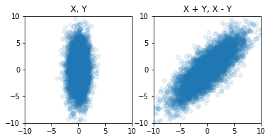
Here is an example of a point set that is negatively correlated – and we can see that if we compute x + y (project on the shown line), the standard deviation on this axis will be lower than on original either x or y:

Putting those together

Let’s put the above identities to action in two simple cases. 

The first one is going to be calculation of mean and variance of average of two variables. We can note (X + Y) / 2 as X / 2 + Y / 2. We can see that the E((X + Y) / 2) will be just (E(X) + E(Y)) / 2, but the variance is var(X)/4 + var(Y)/4 + cov(X, Y)/2.

If var(X) == var(Y) and cov(X, Y) == 0, we get the familiar formula of var(X) / 2 – linear variance scaling.

The second one is a formula of transforming covariances. If we apply a transformation matrix A to our variance/covariance matrix, it becomes A cov(X) A^T. I won’t derive it, but it is a direct application of all of the above formulas and re-writing it in a linear algebra form. What I like about it is the neat geometric interpretation – and relationship to the Gram matrix. I have looked at some of it in my post about image gradients.

Expressing covariance in matrix form is super useful in many fields – from image processing to robotics (Kalman filter!)

Typical noise assumptions

With some definitions and simple linear behaviors clarified, it’s worth to quickly discuss what kind of noise / random variable we’re going to be looking at in computer graphics or image processing. Most denoisers assume AWGN – additive, white, Gaussian noise.

Let’s take it piece by piece:

• Additive – means that noise is added to the original signal (and not for example multiplied),
• White – means that every pixel gets “corrupted” independently and there are no spatial correlations,
• Gaussian – assumption of normal (Gaussian) distribution of noise on each pixel.

Why is this a good assumption? In practice, Poisson noise from counting photons can reasonably resemble an additive Gaussian distribution – and we count every pixel separately.

The same is not true for electrical measurement noises – there are many non-Gaussian components, there are some mild spatial noise correlations resulting from shared electric readout circuitry – and while some publications go extensively into analyzing it, assumption of white Gaussian is “ok” for all but extremely low light photography use-cases. When adding or averaging a lot of different noisy components (and there are many in electric circuitry), the sum eventually gets close enough to Gaussian due to the Central Limit Theorem.

For dithering noise, we typically inject this noise ourselves – and know if it’s white, blue, or not noise at all (patterns like Bayer). Similarly we know if we’re dealing with uniform, or (preferred) triangular distribution – which is not Gaussian, but gets “close enough” for similar analysis.

When analyzing noise from Monte Carlo integration, all bets are off. This noise is definitely not Gaussian, depending on the sampling scheme, sampled functions, most often non white, and generally “weird”. One advantage Monte Carlo denoisers have is strong priors and the use of auxiliary buffers like albedo or depth to guide the denoising – which provides such a powerful additional signal that it usually compensates for the noise characteristics “weirdness”. Note however that if we were to measure its empirical variance, all methods and transformations described here would work the same way.

In all of the uses described above, we initially assume that the noise is zero-mean – expected value of 0. If it wasn’t, it would be considered as the bias of the measurement. All the above linear transformations (adding zero mean noises, multiplying zero mean etc) preserve it. However, we will see now how even zero mean noise can result in non-zero mean and bias after other common transformations.

Including nonlinearities – surprising (or not?) behavior

Let’s start with a quiz, how would you compare the brightness of the three images below:

Central image is clean, the left one has noise added in linear space, the right one in gamma space – noise magnitude is small (as compared to signal) and the same between two images.

This is not a tricky human vision system question – at least I hope I’m not getting into some perceptual effects where display and surround variables twist the results – but I see the image on the left as significantly darker in the shadows as compared to the other two ones – which are hard to compare, as in some areas one seems brighter than the other one.

To emphasize this has nothing to do with perception, when computing the numerical average of all three images, it is different as well: 0.558, 0.568, 0.567. The left one is the darkest indeed.

This is something that surprised me a lot the first time I encountered it and internalized it – the choice of your denoising or blurring color / gamma space will affect the real average brightness of the image! This goes the same for other operations like sharpening, convolution etc.

If you denoise, or even blur an image (reducing noise) in linear space, it will be brighter than if you blurred it in gamma space.

Let’s have a look at why that is. Here is a synthetic test – we assume a signal of 0.2 and the same added zero mean noise, one in linear, one in gamma space (sqrt of the signal which was squared before; with a linear ramp below 0 to avoid a sqrt of negative numbers):

Black line marks the measured, empirical mean, and read line marks mean +/- standard deviation. Adding zero mean noise and applying a non-linearity changes the mean of the signal!

It also changes the standard deviation (much higher!) and skews and deforms the distribution – definitely not a Gaussian anymore.

To start building an intuition, think of a bimodal, discrete noise distribution – one that produces values of either -0.04, or 0.04. Now if we add it to a signal of 0.04 and remap with a sqrt nonlinearity, one value will be sqrt(0.0) == 0, the other one sqrt(0.08) ~=0.283. Their average is  ~0.14, significantly below 0.2 of the square root of the same image that would have no noise.

The nonlinearity is “pushing” points on either side further or closer from the original mean, changing it.

Let’s have a look at an even more obvious example – a quadratic function, squaring the noisy signal.

If we square zero mean noise, we obviously cannot expect it to remain zero mean. All negative values will become positive.

Mean change was something that truly surprised me the first time I saw it with the square root / gamma, but looking at the squaring example, it should be obvious that it’s going to happen with non-linear transformations.

Change of variance / standard deviation should be much more expected and intuitive, possibly also just the change of the overall distribution shape.

But I believe this mean change effect is ignored by most people who apply some non-linearities to noisy signals – for example when dithering and trying to compensate for the sRGB curve that would be potentially applied on writing to a 8bit buffer. If you dither a linear signal, but save to a sRGB texture – you will not only introduce varying noise depending on the pixel brightness (more in the shadows) and be unable to find optimal value – it will be either too small in highlights, or too large in the shadows, but also and even worse – shift the brightness of the image in the darkest regions!

We would like to understand the effects of non-linearities on noise, and in some cases to compensate for it – but to do it, first we need a way of analyzing what’s going on.

We will have a look at three different relatively simple methods to model (and potentially compensate for) this behavior.

Nonlinearity modeling method one – noise transformation Monte Carlo

The first method should be familiar to anyone in graphics – Monte Carlo and a stochastic estimation.

This method is very simple:

1. Draw N random samples that follow the input distribution,
2. Transform the samples with a nonlinearity,
3. Analyze the resulting distribution (empirical mean, variance, possibly higher order moments).

This is what we did manually with the two above examples. In practice, we would like to estimate the effect of non-linearity applied on a measured noisy signal with different signal means. 

We could enumerate all possible means and standard deviations we are interested in – but in practice, dealing with continuous variables, enumerating all values is impossible – we’d need to create a look-up table – sample and tabulate standard deviation and signal mean ranges, compute empirical mean/standard deviation, and interpolate in between, hoping the sampling is dense enough that the interpolation works.

This approach can be summarized in pseudo-code:

For sampled signal mean m
  For sampled noise standard deviation d
    For sample s
      Generate sample according to s and d
      Apply non-linearity
      Accumulate sample / accumulate moments
    Compute desired statistics for (m, d)

This is the approach we used in our Handheld Multi-frame Super-resolution paper to analyze the effect of perceptual remapping on noise. In our case, due to the camera noise model (heteroscedastic Gaussian as an approximation of mixed Gaussian + Poisson noise) our mean and standard deviations were correlated, so we could end up with just a single 1D LUT. In robustness/rejection shader, we would look-up the pixel brightness value, and based on it read the expected noise (standard deviation and mean) from a LUT texture using hardware linear interpolation.

Normally you would want to use “good” sampling strategy – low discrepancy sequences, stratification etc. – but this is beyond the topic of this post. Instead, here is the simplest possible / naive implementation for the 1D case in Python:

def monte_carlo_mean_std(orig_mean: float,
                         orig_std: float,
                         fun : Callable[[np.ndarray], np.ndarray],
                         sample_count: int = 10000) -> Tuple[float, float]:
  samples = np.random.normal(size=sample_count) * orig_std + orig_mean
  transformed = fun(samples)
  return np.mean(transformed), np.std(transformed)

Let’s have a look at what happens with the two functions used before – first sqrt(max(0, x)):

The behavior around 0 is especially interesting:

We observe both an increase in standard deviation (more noise) as well as a significant mean shift. Our signal with mean originally starting at 0 after the transformation starts way above 0. The effect on mean minimizes once we go higher and curves converge, but the standard deviation decreases instead – we will have a look at why in a second.

But first, let’s have a look at the second function, squaring:

And zoomed in behavior around 0:

Here behavior around 0 isn’t particularly insightful – as we expected, mean increases, and the standard deviation is minimal. However when we look at the unzoomed plot, some curious behavior emerges – it looks like the plot of the standard deviation is +/- linear. Coincidence? Definitely not! And we’ll have a look at why – while describing the second method.

Nonlinearity modeling method two – Taylor expansion

When you can afford it (for example, you can pre-tabulate data, deal with only univariate / 1D case etc), Monte Carlo simulation is great. On the other hand, it suffers from the curse of dimensionality and can get very computationally expensive to get reliable answers. Sampling all possible means / standard deviations becomes impractical and prone to undersampling and being noisy / unreliable itself.

The second analysis method relies on the very common engineering and mathematical practice – when you need to know only “approximate” answers of certain “well behaved” functions – linearization, or more generally – Taylor series expansion. 

The idea is simple – once you “zoom-in”, many common functions can resemble tiny straight lines (or tiny polynomials) – where the more you zoom-in on a continuous function, the closer it resembles a polynomial.

What happens if we treat the analyzed non-linear function as a locally linear or locally polynomial and use it to analyze the transformed moments from the direct statistical moment definitions? We end up with neat, analytical formulas of the new transformed statistical moment values!

Wikipedia has some of the derivations for the first two moments (mean and variance).

Relevant formulas for us – second order approximation of mean and the first of variance – are: and .

Let’s have a look at those and try to analyze them before using them.

The first observation is that the mean doesn’t change based on the first derivative of the function, only on the second one (plus obviously further terms). Why? Because the linear component is anti-symmetric around the mean – so the influences on both sides cancel out. This will be generally true for even/odd powers.

The second observation is that if we apply those formulas to the linear transformation a * x, we get the exact formulas – because the linear approximation perfectly “approximates” the linear function.

Variance scaling quadratically with the first derivative (plus error / further terms) is exactly what we expected! Also from this perspective, the above plots of the Monte Carlo of the quadratic function transformed statistical moments makes perfect sense (dx^2 / dx == 2x) – standard deviation will scale linearly with signal strength.

We could compute derivatives manually when we know them – and you probably should, writing for numerical stability, optimal code, and preventing any singularities. But you can also use the auto differentiating frameworks to write once and experiment with different functions. We can write the above as small Jax code snippet:

def taylor_mean_std(orig_mean: float,
                    orig_std: float,
                    fun : Callable[[jnp.ndarray], jnp.ndarray]) -> Tuple[float, float]:
  first_derivative = jax.grad(fun)(orig_mean)
  second_derivative = jax.grad(jax.grad(fun))(orig_mean)
  orig_var = orig_std * orig_std
  taylor_mean = fun(orig_mean) + orig_var * second_derivative / 2.0
  var_first_degree = orig_var * np.square(first_derivative)
  var_second_degree = -np.square(second_derivative) * orig_var * orig_var / 4.0
  taylor_var = var_first_degree + var_second_degree
  return taylor_mean, np.sqrt(np.maximum(taylor_var, 0.0))

And we get almost the same results as Monte Carlo:

This shouldn’t be a surprise – quadratic function is approximated perfectly by a 2nd degree polynomial, because it is a 2nd degree polynomial.

For such an “easy”, smooth, continuous use-cases with convergent Taylor series, this method is perfect – closed formula, very fast to evaluate, extends to multivariate distributions and covariances.

However, if we look at sqrt(max(0, x)) we will see in a second why it might not be the best method for other use-cases.

If you remember how derivatives of the square root look like (and that a piecewise function is not everywhere differentiable) you might predict what the problem is going to be, but let’s look first at how poor approximation it is as compared to Monte Carlo:

The approximation of mean is especially bad – going towards negative infinity.

d/dx(sqrt(x)) = 1/(2 sqrt(x)), and the second derivative d/dx((dsqrt(x))/(dx)) = -1/(4 x^(3/2)). Both will go towards infinity / negative infinity at 0 – and the square root is “locally vertical” around zero!

Basically, Taylor series is very poor at approximating the square root close to 0:

I generated the above plot also using Jax (it’s fun to explore the higher order approximations and see how they behave):

def taylor(a: float,
           x: jnp.ndarray,
           func: Callable[[jnp.ndarray], jnp.ndarray],
           order: int):
  acc = jnp.zeros_like(x)
  curr_d = func
  for i in range(order + 1):
    acc = acc + jnp.power(x - a, i) * curr_d(a)  / math.factorial(i)
    curr_d = jax.grad(curr_d)
  return acc

Going back to our sqrt – for example at 0.001, the first derivative of sqrt is 15.81. At 0.00001, it is 158.11.

With local linearization (pretending only 1st component of the Taylor series matters), this would mean that the noise standard deviation would get boosted by a factor of 158, or variance by 25000!

And the above ignores the effect of “clamping” below 0 -> with a standard deviation of 0.1 and signal means of comparable or smaller magnitudes, many original samples will be negative, and the square root Taylor series obviously doesn’t know anything about it and that we used a piecewise function.

Other than the quality of Taylor series approximation that can be poor for certain functions, to get reliable results we would need to make sure that the noise standard deviation is significantly smaller than the local derivative.

I’ll remark here on something seemingly unrelated. Did you even wonder why Rec. 709 OETF (the same with sRGB) has a linear segment?

This is to bound the first derivative! By limiting the maximum gain to 4.5, we also bound how much noise can get amplified and avoid nasty singularities (a derivative that goes towards infinity). This can matter quite a lot in many applications – and the effect on local noise amplitude is one of the factors.

Even simpler case where Taylor series approximation breaks is “rectified” noise remapping, simple max(x, 0):

Not surprisingly, with such a non-smooth, piecewise function, derivative above 0.0 (equal simply to 1.0) doesn’t tell us anything about the behavior below 0.0 and is unable to capture any of changes of mean and standard deviation…

Overall, Taylor expansion can work pretty well – but you need to be careful and check if it makes sense in the used context – is the function well approximated by a polynomial? Is the noise magnitude significantly smaller than the local standard deviation?

Nonlinearity modeling method three – Unscented transform

As the final “main” method, let’s have a look at something that I have heard of only a year ago from a coworker who mentioned this in passing. The motivation is simple and in a way graphics-related.

If you ever did any Monte Carlo in rendering, I am sure you have used importance sampling – a method of strategically drawing and weighting samples that resembles the analyzed function as close as possible to reduce the Monte Carlo error / variance.

Importance sampling is unbiased, but its most extreme, degenerate form sometimes used in graphics – most representative point (see Brian Karis’s notes and linked references) is biased – as it takes only a single sample and always the same. This is extreme – approximating the whole function with just one sample! One would expect it to be a very poor representation – but if you pick a “good” evaluation point, it can work pretty well.

In math and probability, there is a similar concept – unscented transform. The idea is simple – for N dimensions, pick N+1 sample points (extra degree of freedom needed to compute mean), transform them through non-linearity, and then compute the empirical mean and variance. Yes, that simple! It has some uses in robotics and steering systems (in combination with Kalman filter) and was empirically demonstrated to work better than linearization (Taylor series) for many problems.

Jeffrey Uhlman (author of the unscented transform) proposed a method of finding the sample points through a Cholesky decomposition of the covariance matrix, and for example in 2D those points are: 

In 1D, points are two and trivial – mean +/- standard deviation.

Thus, the code to compute this transformation is also trivial:

def unscented_mean_std(orig_mean: float,
                       orig_std: float,
                       fun : Callable[[np.ndarray], np.ndarray]) -> Tuple[float, float]:
  first_point = fun(orig_mean - orig_std)
  second_point = fun(orig_mean + orig_std)
  mean = (first_point + second_point) / 2.0
  std = np.abs(second_point - first_point) / 2.0
  return mean, std

For the square function, results are almost identical to MC simulation (slightly deviating around 0):

For the challenging square root case, in large range it is pretty ok and close:

However if we zoom-in around 0, we see some differences (but no “exploding” effect):

I marked with the black line the original standard deviation – pretty interesting (but not surprising?) that this is where it starts to break – but always remaining stable.

The max(x, 0) case while not perfect – is also much closer:

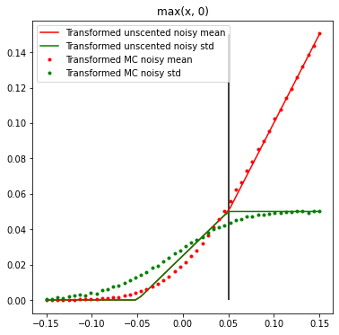
Unscented transform is similar to biased, undersampled Monte-Carlo – it will miss behavior beyond +/- standard deviation, and also undersample between two evaluation points – but should work reasonably well for a wide variety of cases.

I will return to final recommendations in the post summary, but overall if you don’t have a huge computational budget and analyzed non-linear functions don’t behave well, I highly recommend this method.

Bonus nonlinearity modeling methods – analytical distributions

The final method is not a single method, but a general observation.

I am pretty sure most of my blog readers (you, dear audience 🙂 ) are not mathematicians and I’m not one either – even if we use a lot of math in our daily work and many of us love it. When you are not an expert of a domain (like probability theory), it’s very easy to miss solutions to already solved problems and try reinventing them.

Statistics and probability theory analyze a lot of distributions, and a lot of transformations of those distributions with closed formulas for mean, standard deviation and even further moments.

One example would be a rectified normal distribution and truncated normal distribution.

Those distributions can very easily arise in signal and image processing (if we miss information about negative numbers) – and there are existing formulas for their moments analyzed by mathematicians. One of my colleagues has successfully used it in extreme low light photography to remove some of the color shifts resulting from noise truncation during processing.

This is a general advice – it’s worth doing some literature search outside of your domain (can be challenging due to different terminology) and asking around – as it might have been a solved problem.

Practical recommendation and summary

In this post I have recapped effects of linear transformations of random variables, and described three different methods of estimating effects of non-linearities on the basic statistical moments – mean and variance/standard deviation.

This was a more theoretical and math heavy post than most of mine, but it is also very practical – all of those three methods were things I needed (and have successfully used) at work.

So… from all three, what would be my recommendation? 

As I mentioned, I have used all of the above methods in shipping projects. The choice of particular one will be use-case dependent – what is your computational budget, how much you can precompute, and most importantly – how your non-linearities look like – the typical “it depends”.

If you can precompute, have the budget, and used functions are highly non-linear and “weird”? Use Monte Carlo! Your non-linear functions are almost polynomial and “well behaved”? Use the Taylor series linearization. A general problem and a tight computational budget? I would commonly recommend the unscented transform.

…I might come back to the topic of noise modeling in some later posts, as it’s both a very practical and very deep topic, but that’s it for today – I hope it was insightful in some way.