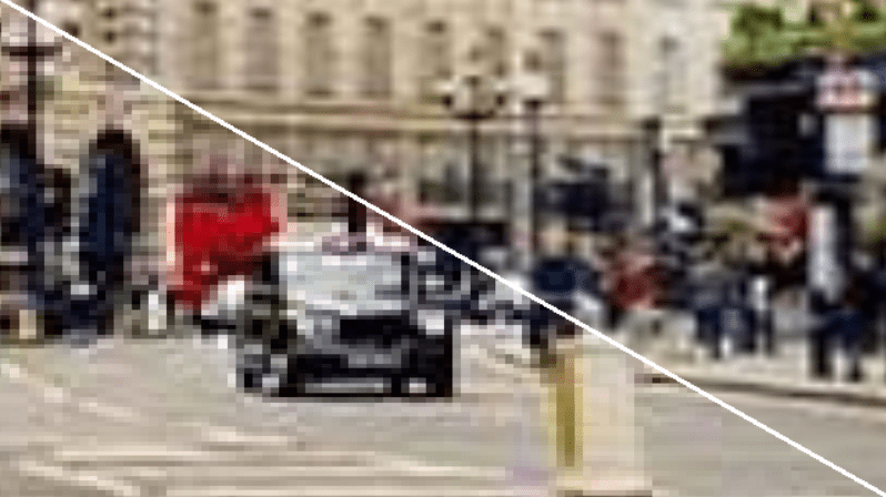
In this post we will look at one of the staples of real-time computer graphics – bilinear texture filtering. To catch your interest, I will start with focusing on something that is often referred to as “bilinear artifacts”, trapezoid/star-shaped artifact of bilinear interpolation – what causes them? I will discuss briefly some common bilinear filtering alternatives and how they fix those, link a few of my favorite papers on (fast) image interpolation, and analyze the frequency response of common cheap filters.

As usual, I will work on the topic in “layers”, starting with basics and “introduction to graphics” level and perspective – analyzing the “spatial” side of the artifact. Then I will (non-exhaustively) the alternatives – bicubic and biquadratic filter, and finally analyze those from a signal processing / EE / Fourier spectrum perspective. I will also comment on relationship between filtering as used in the context of upsampling / interpolation, and shifting images. (Note: I am going to completely ignore here downsampling, decimation, and generally trilinear filtering / mip-mapping.)

Update: Based on a request, I added a link to a colab with plots of the frequency responses here.

What is bilinear filtering and why graphics use it so much?

I assume that most of the audience of my blog post are graphics practitioners or enthusiasts and most of us use bilinear filtering every day, but a quick recap never hurts. Bilinear filtering is a texture (or more generally, signal) interpolation filter that is separable – it is a linear filter applied on the x axis of the image (along the width), and then a second filter applied along the y axis (along the height).

Note on notation: Throughout this post I will use linear/bilinear almost interchangeably due to this property of bilinear filtering being a linear filter applied in the two directions sequentially.

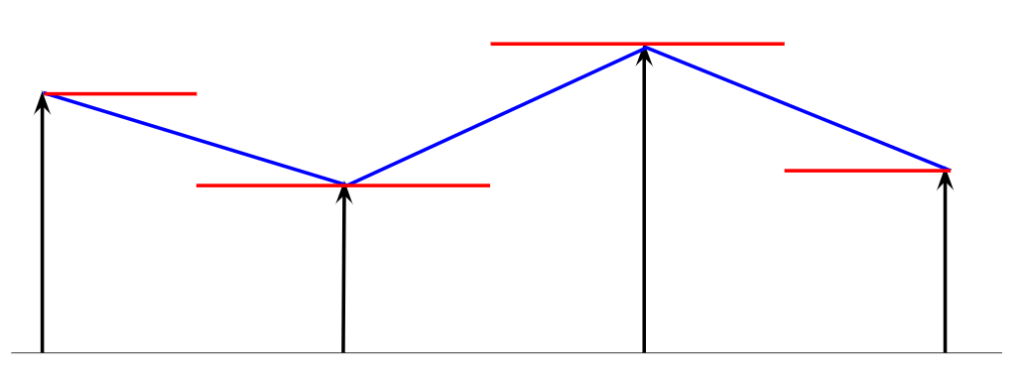
Starting with a single dimension, linear filter is often called a “tent” or “triangle” filter. In the context of input texture interpolation, we can look at it as either “gather” (“when computing an output pixel, which samples contribute to it?”), or “scatter” operation (“for each input sample, what are its contributions to the final result?”). Most of GPU programmers naturally think of “gather” operations, but here this “triangle” part is important, so let’s start with the scatter.

For every input pixel, its contributions to the output signal form a “tent” – a “triangle” of pixel contributions is centered at sample N, with height equal to the sample/pixel N value, and its base spans from the sample (N-1) to (N+1). To get the filtering result we sum all contributing “tents” (there are either 1 or 2 covering each output pixel). All of triangles have the same base length, and all of them overlap with a single other triangle on either side of the top vertex. Here is a diagram that hopefully will help:

Switching from “scatter” to a more natural (at least to people who write shaders) gather approach – between samples (N+1) and (N) we sum up contributions of all “tents” covering this area, so (N+1) and N, and at exact position of the sample N we get only its contribution.

Formula for this line is simply xn * (t – 1) + xn-1 * t. This means that in 1D each output sample has two contributing input pixels (though sometimes one contribution is zero!), and we linearly interpolate between them. If we repeat this twice per x and y, we end up with four input input samples and four weights (t_x – 1) * (t_y – 1), (t_x ) * (t_y – 1), (t_x – 1) * (t_y ), (t_x) * (t_y). Since the weights are just multiplication of independent x and y weights, we can verify that this filter is separable (if you are still unsure what it means in practice, check out my previous blog post on separable filters).

Bilinear filtering is ubiquitous in graphics and there are a few reasons for it – but the main one is that is super cheap, and furthermore, hardware accelerated; and that it provides significant quality improvement over nearest-neighbor filtering.

All modern GPUs can do bilinear filtering of an input texture in a single hardware instruction. This involves both memory access (together with potentially uncompressing block compressed textures into local cache), as well as the interpolation arithmetic. Sometimes (depending on the architecture and input texture bit depth) the instruction might have slightly higher latency, but unless someone is micro-optimizing or has a very specific workload, the cost of the bilinear filtering can be considered “free” on contemporary hardware.

At the same time, it provides significant quality improvement over “nearest neighbor” filtering (just replicating each sample N times) for low resolution textures.

Being supported natively in hardware is a huge deal and the (bilinear) texture filtering was one of the main initial features of graphics accelerators (when they were still mostly separate cards, in addition to the actual GPUs).

Personal part of the story – I still remember the day when I saw a few “demo” games on 3dfx Voodoo accelerator on my colleague’s machine (it was a Diamond Monster3D) back in primary school. Those buttery smooth textures and no pixels jumping around made me ask my father over and over again to get us one (at that time we had a single computer at home, and it was my father’s primary work tool) – a dream that came true a bit later, with Voodoo 2.

Side remark – pixels vs filtering, interpolation, reconstruction

One thing that is worth mentioning is that I deliberately don’t want to draw input – or even the output pixels as “little squares” – pixels are not little squares!

Classic tech memo from Alvy Ray Smith elaborates on it, but if you want to to deeper into understanding filtering, I find it extremely important to not make such a “mistake” (I blame “nearest neighbor” interpolation for it).

So what are those values stored in your texture maps and framebuffers? They are infinitely small samples taken at a given location. Between them, there is no signal at all – you can think of your image as “impulses”. Such signal is not very useful on its own, it needs a reconstruction filter that reconstructs a continuous, non discrete representation. Such a reconstruction filter can be your monitor and in this case, pixels could be actually squares (though different LCD monitors have different pixel patterns), or a blurred dot of a diffracted ray in CRT monitor. (This is something that contemporary pixel art gets wrong and Timothy Lottes used to have interesting blog posts about – I think they might have gotten deleted, but his shadertoy showing more correct emulation of a CRT monitor is still there).

For me it is also useful to think of texture filtering / interpolation in a similar way – we are reconstructing a continuous (as in – not discrete/sampled) signal and then resample it, taking measurements / values at new pixel positions from this continuous representation. This idea was one of key components in our handheld mobile super-resolution work at Google, allowing to resample reconstructed signals at any desired magnification level.

Bilinear artifacts – spatial perspective – pyramid, and mach bands

Ok, bilinear filtering seems to be “pretty good” and for sure is cheap! So what are those bilinear artifacts?

In the post intro I have shown example artifact from a 20 year old video game back when the asset textures were very low resolution, but those happen anytime we interpolate from low resolution buffers. In my Siggraph 2014 talk about volumetric atmospheric effects rendering, I have shown an example of problematic artifacts when upsampling low resolution 3D fog texture:

In my old talk proposed to solve this problem with additional temporal low-pass effect (temporal jitter + temporal supersampling), because the alternative (bicubic / B-spline sampling – more about it later) was too expensive to apply in real time. Nota bene such a solution is actually pretty good at approximating blurring / filtering for free if you already have a TAA-like framework.

If we get back to our “tent” filter scatter interpretation, it should become easier to see what causes this effect. Separable filtering applies first a 1D triangle filter in one direction, then in another direction, multiplying the weights. Those two 1D ramps multiplied together result in a pyramid – this means that every input pixel will “splat” a small pyramid, and if the ratio of the output to the input resolutions is large and textures have high contrast, then those will become very apparent. Similarly those pyramids on any edge that is not aligned with perfect 45 degrees, will create jaggy, aliased appearance.

Ok, it’s supposed to be a pyramid, but what’s the deal with this bright star-like lines?

The second “spatial” effect of why bilinear filtering is not great are so-called Mach bands.

This phenomenon is one of the fascinating “artifacts” (or conversely – desired features / capabilities) of human visual system. Human vision cannot be thought of as a “sensor” like in a digital camera or “film” in analog one – it is more like a complicated video processing system, will all sorts of edge detectors, contrast boosting, motion detection, embedded localized tonemapping etc. Mach bands are caused by tendency of HVS to “sharpen” image and emphasize any discontinuity.

(Bi)linear interpolation is continuous, however its derivative is not (derivative of a piecewise linear function is a piecewise constant function). In mathematical definition of smoothness and C-continuity we say that it is C0 continuous, but not C1 continuous. I find it fascinating that HVS can detect such discontinuity – detecting features like lines and corners is like differentiation and indeed, most common and basic feature detector in computer vision, Harris Corner Detector analyzes local gradient fields.

To get rid of this effect, we need some filtering and interpolation that has a higher order of continuity. Before I move to some other filters, I have to mention here also a very smart “hack” from Inigo Quilez – by hacking the interpolation coordinates, you can get interpolation weights that are C1 continuous.

It’s a really cool hack and works very well with procedural art (where manually computed gradients are used to produce for example normal maps), but produces “rounded rectangles” type of look and aliases in motion, so let’s investigate some other fixes.

Bilinear alternatives – bicubic / biquadratic

The most common alternative considered in graphics is bicubic interpolation. The name itself is in my opinion confusing, as cubic filtering can mean any filtering where we use 4 samples, and filter weights result from evaluating 3rd order polynomials (similarly to linear using 2 samples and a 1st order polynomial). In 2D, we have 4×4 = 16 samples, but we also interpolate separably. However there are many alternative 3rd order polynomials weights that could be used for filtering… This is why I avoid using just the term “bicubic”. Just look at Photoshop image resizing options, does this make any sense!?

The most common bicubic filter used in graphics is one that is also called B-Spline bicubic (after reading this post, see this classic paper from Don Mitchell and Arun Netravali that analyzes some other ones – I revisit this paper probably once every two months!). It looks like this:

As you can see, it is way smoother and seems to reconstruct shapes much more faithfully than bilinear! Smoothness and lack of artifacts comes from its higher order continuity – it is designed to have matching and continuous derivatives at each original sample point.

It has a few other cool and useful properties, but my personal favorite one is that because all weights are positive, it can be optimized to use just 4 bilinear samples! This old (but not dated!) article from GPU Gems 2 (and a later blog post from Phill Djonov elaborating on the derivation) describe how to do it with just some extra ALU to compute the look-up UVs. (Similarly in 1D this can be done in just 2 samples – which can be quite useful for low-dimensionality LUTs).

Its biggest disadvantage – it is visibly “soft”/blurry, looks like the whole image got slightly blurred – which is what is happening… Some other cubic interpolators are sharper, but you have to pay a price for that – negative filter weights that can cause halos / ringing, as well as make it impossible to optimize so nicely.

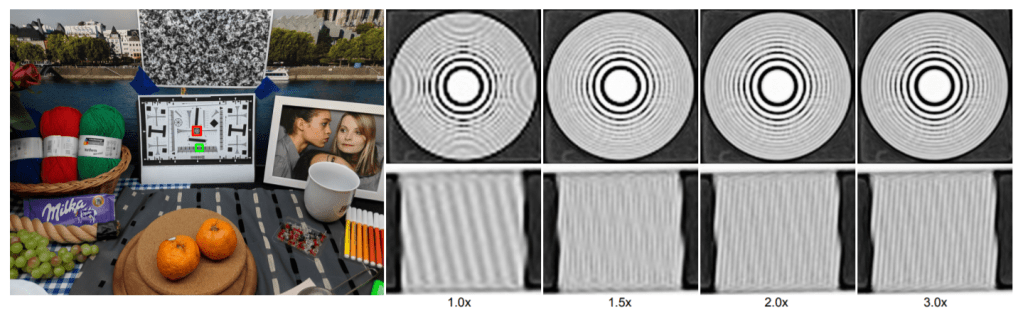
Second alternative that caught my attention and was actually a motivation to finally write something about image resampling was a recent blog post from Thomas Deliot (and an efficient shadertoy implementation from Leonard Ritter) on biquadratic interpolation – continuous interpolation that reconstructs a quadratic function and considers 3 input samples (or 9 in 2d). I won’t take the spotlight from them on how it works, I recommend checking the linked materials, but included an animated comparison – it looks very good, sharper than the bspline bicubic, and is a bit cheaper.

Post update: Won Chun pointed to me a super interesting piece of literature on quadratic filters from Neil Dogson. The link is paywalled, but you will easily find references by googling for “Quadratic interpolation for image resampling”. It derives the quadratic filter with an additional parameter that allows to control filter sharpness similarly to bicubic filters parameters B/C. The one that I used for analysis is the blurriest, “approximating” one. Here is a shadertoy from Won Chun and a corresponding Desmos calculator that proposes also a 2 sample approximation of the (bi)quadratic filter, cool stuff!

Interpolation – shifting reconstructed signal and position dependent filtering

A second perspective that I am going to discuss here is how texture filtering creates different local filters and filter weights depending on the fractional output/input pixel positions relationship.

Let’s consider for now only 1D separable interpolation and the range of 0.0-0.5 (-0.5 to 0.0 or 0.5 to 1.0 can be considered as switching to different sample pair, or symmetric).

With a subpixel offset of 0.0, linear weights will be [1.0, 0.0], and with a subpixel offset of 0.5, they will be [0.5, 0.5]. Those two extremes correspond to a very different image filters! Imagine input filtered with a convolution filter of 1 (this returns just the original one) vs a filter of [0.5, 0.5] – this corresponds to low quality, box blur of the whole image.

To demonstrate this effect, I made a shadertoy that compares bilinear, bicubic bspline, biquadratic, and a sinc filter (more about it later) with dynamically changing offsets.

So with an offset of U or V of 0.5, we are introducing very strong blurring (even more with both shifted – see above), and no blurring at all with no fractional offsets.

Knowing that our effective image filters change based on the pixel “phase” we can have a look at spectral properties and frequency responses of those filters and see what we can learn about those resampling filters.

Bilinear artifacts – variance loss, and frequency perspective

So let’s have a look at filter weights of our 3 different types of filters as they change with pixel phase / fractional offset:

As expected, they are symmetric, and we can verify that they sum to 1. Weights are quite interesting themselves – for example quadratic interpolation with fractional offset of 0.0 has the same filter weights as the linear interpolation with offset of 0.5!

Looking at fractional offset dependent, we can analyze how those weights affect the signal variance, as well as the frequency response (and in effect, frequency content of the filtered images). Variance change resulting from a linear filter is equal to the sum of the squares of all its weights. So let’s plot the effect on input signal variance from those three filters.

With the bilinear filter, the total variance changes (a lot!) with the subpixel position – which will cause apparent contrast loss. Variance and contrast loss due to blending/filtering is an interesting statistical effect, very visible perceptually, and one of my favorite papers on procedural texture synthesis from Eric Heitz and Fabrice Neyret achieves very good results from blending random blended tilings of an input texture mostly “just” by designing a variance preserving blending operator!

Now, moving to the full frequency response of a those filters – for this we can use for example Z-transform commonly used in signal processing (or go directly with complex phasors). This is goes beyond scope of this blog post, (if you are interested in details, let me know in the comments!) but I will present the resulting frequency responses of those 3 different filters:

Looking at those plots we can observe a very different behavior. As we realized above, linear at no fractional offset produces no filtering effect at all (identity response), and both other filters are lowpass filters. Interestingly, no offset is where quadratic interpolation performs the most lowpass filtering, the opposite of both other filters! To be able to reason about the filters in more of isolation, I also plotted each filters frequency response at different phases on a single plot for each:

Looking at these plots, we can see that bspline cubic is the most “consistent” between the different fractional offsets, while quadratic is less consistent, but filters out somewhat less of high frequencies (which is part of its sharper look). Linear is the least consistent, going from between a very sharp image, and a very blurry one.

This inconsistency (both in terms of total variance, as well as frequency response – in fact the first can be derived from the latter from Parseval’s theorem) is another look at what we perceive as bilinear artifacts – “pulsing” and inconsistent filtering of the image. Looking at linear image shifted with phase 0.0 and 0.5 is like looking at two very different images. While bicubic bspline over-blurs the input, it is consistent, doesn’t “pulse” with changing offsets and doesn’t create aliased visible patterns. I see the biquadratic filter as kind of a “middle ground” that looks very reasonable and definitely will use it in practice.

Given how bicubic and similar filters have quite consistent lowpass filtering, some of the blurring effect can be compensated with an additional, sharpening filter. This is what for example my friend Michal Drobot proposed in his talk on TAA for Far Cry 4 (and others have arrived to and used independently) – after resampling, do a global uniform sharpening pass on the whole image to counter some of the blurriness. Given how blurriness is relatively constant, sharpen filter can be even designed to recover the missing input frequencies accurately!

Bilinear / bicubic alternatives – (windowed) sinc

It’s worth noting that resampling filters don’t have to necessarily so heavily blur out the images and their frequency response can be much more high frequency preserving. This is beyond scope of this blog post, but some bicubic filters are actually designed to be slightly sharpening and boosting some of the high frequencies (Catmull-Rom spline – often used in TAA for continuous resampling).

Such built-in sharpening might not be desired, so many filters are designed to be as frequency preserving as possible (windowed sinc like Lanczos). As I mentioned, it is beyond the scope of this blog post, but just for fun, I include example frequency response of a truncated (non windowed!) sinc, as well as final gif comparison. Such a sinc is also featured in my shadertoy.

For much more complete and comprehensive treatment of filter trade-offs (sharpness, ringing, oversharpening), I again highly recommend this classic paper from Mitchell and Netravali – be sure to check it out.

Conclusions

This post touched on lots of topics and connection between them (I hope that it could be inspiring for you to go deeper into them) – I started with analyzing the most common, simple, ardware accelerated image interpolation filter – bilinear. I discussed its limitations and why it is often replaced (especially when interpolating from very low resolution textures) by other filters like bicubic – which might seem counter-intuitive given that they are much blurrier. I discussed what causes the “bilinear artifacts”, both from the simple spatial filtering perspective, as well as the effect of variance loss / contrast reduction / lowpass filtering. I barely scratched surface of the topic of interpolation, but I had fun writing it (and creating the visualizations), so expect some follow up posts about it in the future!