

In this post, we’ll have a look at the idea of removing blur from images, videos, or games through a process called “deconvolution”.
We will analyze what makes the process of deblurring an image (blurred with a known blur kernel) – deconvolution – possible in theory, what makes it impossible (at least to realize “perfectly”) in practice, and what a practical middle ground looks like.
Simple deconvolution is easy to understand, and it connects very nicely pure intuition, linear algebra, as well as frequency domain and spectral matrix analysis.
In the second part of the post we will look at how to apply efficient approximate deconvolution using only some very simple and basic image filters (gaussians) that work very well in practice for mild blurs.
Linear image blur – convolution
Before we dive into defining what is “deblurring” (or even going further into deconvolution), let’s first have a look at what is blur.
I had posts about various kinds of blurs, the most common being Gaussian blur.
Let’s stop for a second and look at the mathematical formulation of blur through convolution.
Note: I will be analyzing mostly examples in 1D dimension, calling sequence entries “samples”, “elements”, and “pixels” interchangeably, while also demonstrating image convolutions as 2D (separable) filters. 2D is a direct extension of all the presented concepts in 1D – harder to visualize in algebraic form or frequency plots, but more natural for looking at the images. I hope examples in alternating 1D and 2D won’t be too confusing. Separable filters can be deconvolved separably as well (up to a limit), while non-separable ones not.
“Blur” in “blurry images” can come from different sources – camera lens point spread function, motion blur from hand shake, excessive processing like denoising, or upsampling from lower resolution.
All of those have in common that come from a filter that either “spreads” some information like light rays across the pixels, or alternatively combines information from multiple source locations (whether physical circle of confusion, or nearby pixels). We typically call it a “blur” when all weights are positive (this is the case in physical light processes, but for electric or digital signals not necessarily), and it results in a low-pass filter.
There are two mentioned ways of looking at blurs – “scatter”, where a point contributes into multiple target output elements, and “gather”, where for each destination elements, we look at contributing source points. This is a topic for a longer post, but in our case – where we look at “fixed” blurs shared by all the locations in the image – they can be considered equivalent and transpose of one another (if a source pixel contributes to 3 output pixels, each output pixel also depends on 3 input pixels).
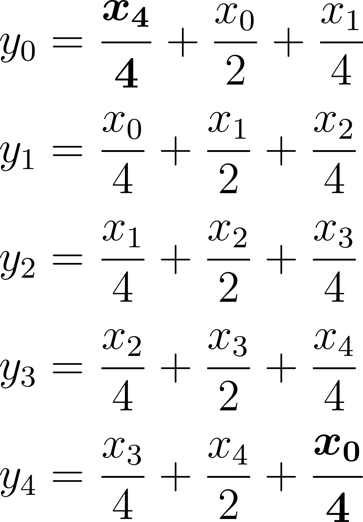
Let’s look at one of the simplest filters, binomial convolution filter [0.25, 0.5, 0.25].
This filter means that given five pixels,  , we have output pixels:

Note that for now we have omitted the output pixels  and it’s not immediately obvious how to treat them; where would we get the missing information from (reading beyond
  )? This relates to “boundary conditions” which matter a lot for analysis and engineering implementation details, and we will come back to it later. Typical choices for “boundary conditions” are wrapping around, mirroring pixels, clamping to the last value, treating all missing ones as zeros, or even just throwing away partial pixels (this way a blurred image would be smaller than the input).
In physical modeling – for example when blur occurs in camera lens – we sample a limited “rectangle” of pixels from a physical process that happens outside, so it’s similar to throwing away some pixels.
Such a simple [0.25, 0.5, 0.25] filter and simple convolution when applied on an image in 2D (first in 1D in horizontal axis and then in 1D in the vertical one, results in a relatively mild, pleasant blur:
But if we had such an image and we knew where the blur comes from and its characteristics… could we undo it?
Deblurring through deconvolution
Process of inverting / undoing a known convolution is called simply deconvolution.
We apply a linear operator to the input… so, can we invert it?
In a fully general case not always (general rules of linear systems apply; not all are invertible!), but “approximately”? Most often yes, and let’s have a look at the math of deconvolution.
But before that, I will clarify a common confusing topic.
Is deconvolution the same as sharpening, super-resolution, upsampling?
No, no, and no.
Deconvolution – process of removing blur from an image.
Sharpening – process of improving the perceived acuity and visual sharpness of an image, especially for viewing it on a screen or print.
Super-resolution – process of reconstructing missing detail in an image.
Upsampling – process of increasing the image resolution, with no relation to blur, sharpness, or detail – but aiming to at least not reduce it. Sadly ML literature calls upsampling “single frame super-resolution”.
Where does the confusion come from?
Other than the ML literature super-resolution confusion, there is overlap between those topics. Sharpening can be used to approximate deconvolution and often provides reasonable results (I will show this around the end of this post). If you did sharpening in Photoshop to save a blurry photo, you tried to approximate deconvolution this way!
Super-resolution is often combined with deconvolution in “CSI” style detail and acuity enhancement pipelines.
Upsampling is often considered “good” when it produces edges with sharper falloff than the original Nyquist and often has some non-linear and deconvolution-like elements.
But despite all that, deconvolution is simply undoing a physical process or pipeline processing of a convolution.
Equations of deconvolution
Let’s have a look at the equations that formed the basis of convolution again:
It should be obvious that we cannot directly solve for any of x variables – we have 3 equations and 5 unknowns…
But if we look at some simple manipulation:
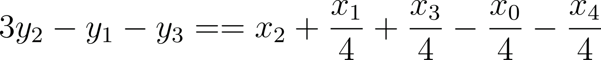
We can see that we get: , where
 ![]() is a residual error (sum of four quartered input pixels)
is a residual error (sum of four quartered input pixels)
If we apply this filter to the blurred image from before we get… an ugly result:
Yes, it is very “sharp”, but… ugh.
It’s clear that we need more “source” data. We need “something” to cancel out those error terms further away…
Note: I did this exercise, as this is important to build intuition and worth thinking about – for full cancellation we will need more and more terms, up to infinity. Anytime we include pixels further away, we can make the residual error smaller (as multiplying by the further weights and iterating this way shrinks them down).
But to solve an inverse of a linear system in general – we obviously need at least as many knowns as unknowns in our system of equations. At least, because linear dependence might make some of those equations cancel out.
This is where boundary conditions and handling of the border pixels comes into play.
One example is “wrap” mode, which corresponds to circulant convolution (we will see in a second why this is neat for mathematical analysis; not necessarily very relevant for practical application though 🙂 ).
Notice the bolded “wrapping” elements. I was too lazy to solve it by hand, so I plugged it into sympy and got:

This is a valid solution only for this specific, small circulant system of equations. In general, we could definitely end up with a non-invertible system – where we lose some degrees of freedom and again have too many unknowns as compared to known variables.
But in this case, if we increase the number of the pixels to 7, we’d get:

There’s an interesting pattern happening… that pattern (sign flipping and adding plus two to a center term) will continue – to me this looked similar to a gradient (derivative) filter and it’s not a coincidence. If you’re curious about the connection, check out my past post on image gradients and derivatives and have it in mind once we start analyzing the frequency response and seeing the gain for the highest frequencies going towards infinity.
For the curious – if we apply such a filter to our image, we get absolutely horrible results:
This got even worse than before.
Instead of toying with tiny systems of equations and wondering what’s going on, let’s solve it by getting a better understanding of the problem and going “bigger” and more general: looking at the matrix form of the system of equations.
Convolution and deconvolution matrix linear algebra
Any system of equations can be represented in a matrix form.
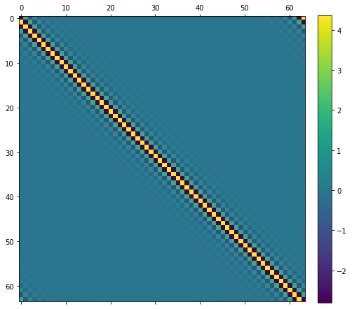
Circulant convolution of 128 pixels will look like this:

Make sure you understand this picture. Horizontal rows are output elements, vertical columns are input elements (or vice versa; row major vs column major, in our case it doesn’t matter, though I am sure some mathematicians would scream reading this). Each row has 3 elements contributing to it – in 1D each output element depends on 3 input elements.
This is a lovely structure – (almost) block diagonal matrix. Very sparse, very easy to analyze, very efficient to operate.
Edit: Nikita Lisitsa mentioned on twitter that this specific matrix is also tridiagonal. Those appear in other applications like 1D Laplacians and are even easier to analyze. More general convolutions (more elements) are not tridiagonal though.
Then to get a solution, we can invert the matrix (this is not a great idea for many practical problems, but for our analysis will work just fine). Why? This linear system transforms from input elements / pixels to output elements pixels. We are interested in the inverse transformation – how to find the input, unblurred pixels, knowing the output pixels.
However, if we try to invert it numerically… we get an absolute mess:
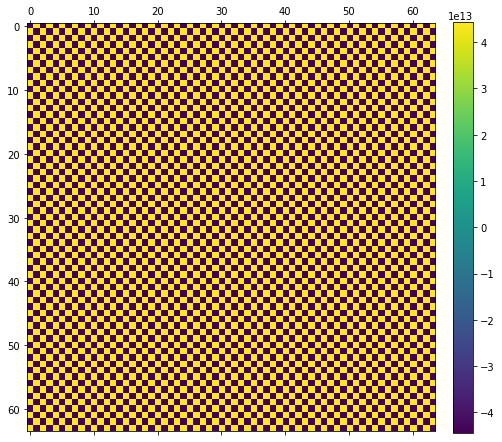
Numpy produces this array: [[-4.50359963e+15, 4.50359963e+15, -4.50359963e+15, …,]]. When we look at the determinant of the matrix, it is close to zero, so we can’t really invert it. I am surprised I didn’t see any actual errors (numerical and linear algebra packages might or might not warn you about matrix conditioning). This means that our system is “underdetermined” (some equations are linearly dependent on each other and there is not enough information in the system to solve for the inverse) and we can’t solve it exactly…
Luckily, we can regularize the matrix inverse by our favorite tool – singular value decomposition. In the SVD matrix inversion, we obtain an inverse matrix by inverting pointwise singular values and transposing and swapping the singular vector matrices.
Singular values look like this:
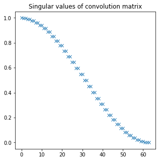
If this reminds you of something… just wait for it. 🙂
But we see that we can’t really invert those singular values that are close to 0.0. This will blow up numerically, up to infinity. If we regularize the inversion (instead of  do for example
  ), we can get a “clean” inverse matrix:
This looks much more reasonable. And if we apply a filter obtained this way (one of the rows) to the blurred image,we get a high quality “deblurred” image, almost perfectly close to the source:
Worth noting: if we had a filter that does somewhat less blur, for example [0.2, 0.6, 0.2], we would get singular values:
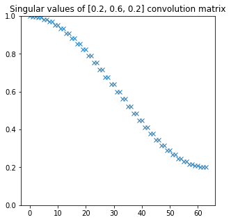
And the direct inversion would be also much better behaved (no need to regularize):

Time to connect some dots and move to a more “natural” (and my favorite) convolution domain – frequency analysis.
Signal processing and frequency domain perspective
Let’s have a look at the frequency response of the original filter. Why? Because we will use Fourier transform and convolution theorem. It states that when performing (inverse or regular) Fourier transform (or its discrete equivalents) convolution in one space is multiplication in the other space.
So if we have a filter response like this:
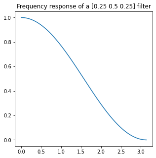
(Looks familiar?)
It will multiply the original frequency spectrum. We can combine linear transforms in any order, so if we want to “undo” the blurring convolution, we’d want to multiply by… simply its inverse.
Here we encounter again the difficulty of inversion of such a response – it goes towards zero. To invert it, we would need to have a filter with response going towards infinity:
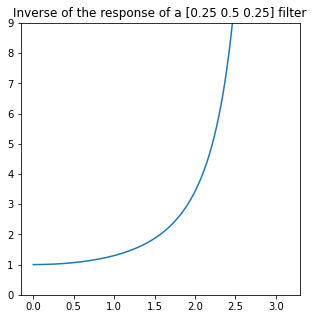
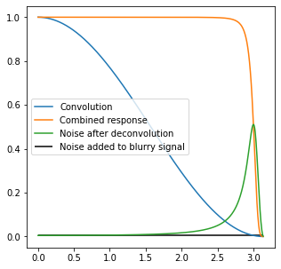
This would be a bad idea for many practical reasons. But if we constrain it (more about the choice of constraint / regularization later), we can get a “reasonable” combined response:
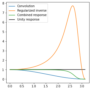
We would like the “combined response” to be a perfect flat unity, but this is not possible (need for an infinite gain) – so something like this looks great. In practice, when we deal with noise, maximum gains of 8 might already be too much, so we would need to reduce it even more.
But before we tackle the “practicalities” of deconvolution, it’s time for a reveal of the connection between the matrix form and frequency analysis.
They are exactly the same.

This shouldn’t be surprising if you had some “advanced” linear algebra at college (I didn’t; and felt jealous watching Gilbert Strang’s MIT linear algebra course – even if you think you know linear algebra, whole course series is amazing and totally worth watching) or played with spectral analysis / decomposition (I have a recent post on it in the context of light transport matrices if you’re interested).
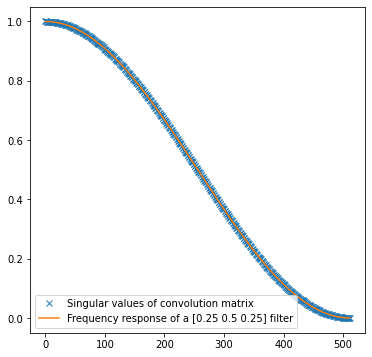
Circulant matrix, such as convolution matrix, diagonalizes as Discrete Fourier Transform. This is an absolutely beautiful and profound idea and analyzing behaviors of this diagonalization was one of the prerequisites for the development of the Fast Fourier Transform.
When I first read about it, I was mind blown. I shouldn’t be surprised – Fourier series and complex numbers appear everywhere. Singular values of a circulant (convolution) matrix are amplitude frequency buckets of the DFT.
This is the reason I picked kind of “unnatural” (for graphics folks) wrapping boundary condition – Fourier transform is periodic and a wrapping cyclic convolution matrix is diagonalized through it. We could have picked some other boundary conditions and the result would be “similar”, but not exactly the same. In practice, it doesn’t matter outside of the borders (where “mirror” would be my practical recommendation for minimizing edge artifacts for blurs; and either “mirror” or “clamp” works well for deconvolution).
This is another way of looking at why some convolution matrices are impossible to invert – because we get frequency response at some frequency buckets equal to zero and therefore the singular values also equal to zero!
Nonlinear, practical reality of deblurring
I hope you love convolution matrices and singular values as much as I do, but if you don’t – don’t worry, time to switch to more practical and applicable information. How can we make simple linear deconvolution work in practice? To answer that, we need to analyze first why it can fail.
Infinite gain
We already discovered one of the challenges. We cannot have an “infinite” gain on any of the frequencies. If some information from singular values / frequencies truly goes to 0, we cannot recover it. Therefore, it’s important to not try to and not invert the frequencies close to zero and constrain the maximum gain to some value. But how and based on what? We will see how noise helps us answering this question.
Noise
The second problem is noise. In photography, we always deal with noisy images and noise is part of the image formation.
If we add noise with standard deviation of 0.005 to the blurry image (assuming signal strength of 1.0), we’re not going to notice it. But see what happens when deconvolving it:
This relates to the gain point before – except that we are not concerned with just “infinite” gains, but any strong gain on any of the frequency buckets will amplify the noise at that frequency… This is a frequency space visualization of the problem:
Notice how the original white noise got transformed into some weird blue-noise (only the highest frequencies) – and we can see this actually on the image, with an extreme checkerboard-like pattern.
Quantization, compression, and other processing
Noise is not the only problem.
When processing signals in the digital domain, we always quantize them. While rendering folks might be working a lot with floats and tons of dynamic range (floats obviously also quantize, but it’s an often forgiving, dynamic quantization), unfortunately camera image signal processing chain, digital signal processors, and image processing algorithms mostly don’t. Instead they operate on fixed point, quantized integers. Which makes a lot of sense, but when we save an image in 8 bits (perfectly fine for most displays) and then try to deconvolve it, we get the following image:

The noise itself is not huge; but in terms of structure, it definitely is similar to the noisy one above – this is not a coincidence.
Quantization can be thought of as adding quantization noise to the original signal. If there is no dithering, this quantization noise is pretty nasty and correlated, with dithering it can be similar to white noise (with known standard deviation). In either case, we have to take it into account to not produce visual artifacts and one can use expected quantization noise standard deviation of  , where
  is a difference between two closest elements due to quantization.
Significantly worse problems can arise from other image processing and storage techniques like compression. Typically a high quality deconvolution from compressed images is impossible using linear filters – but can be definitely achieved with non-linear techniques like optimization or machine learning.
Aliasing
And then, there’s aliasing. The ubiquitous signal processing and graphics problem. The reason it comes up here is that even if we model blur coming from a lens perfectly, then when we sample the signal by camera sensor and introduce aliasing, this aliasing corrupts the measurements of the higher (and sometimes mid or lower!) frequencies of the input signal.
This is beyond the scope of this post, but this is why one would want to do a proper super-resolution and multiframe reconstruction of the signal first – that both removes aliasing, as well as reconstructing the higher frequencies – before any kind of deconvolution. Unfortunately any super-resolution reconstruction error might be amplified heavily this way, so worth watching out.
Different signal space, gamma etc
If blur happens in one space (e.g. photons, light intensity), then deblurring in another space (gamma corrected images) is a rather bad idea. It can work “somewhat”, but I’d recommend against doing so. Interestingly, my recommendation is at odds with the common practice of sharpening (for appearance) in the output space (“perceptual”) which tends to produce less over-brightening – while convolution happens in the linear light space. I will ignore this subtlety here, and simply recommend deconvolving in the same space as the convolution happened.
Regularizing against noise and infinities
What can we do about the above in practice? We can always bound the gain to some maximum value and find it by tuning. That can work ok, but feels inelegant and is not noise magnitude dependent.
An alternative is Wiener deconvolution which provides a least-squares optimal estimation of the inverse of a noisy system. Generally, Wiener filter requires knowing the power spectral density distribution of the input signal. We could use the image / signal empirical PSD, or general, expected distribution for natural images. But I’ll simplify even further and assume a flat PSD of 1 (not correct for natural images that have a strong spectral decay!), getting a formula for a general setting with response of  , where X is a convolution filter frequency response, and
  is per frequency noise standard deviation. Wikipedia elegantly explains how this can be rephrased in terms of SNR:

With infinite or large SNR, this goes towards direct inverse. With tiny SNR, we get cancellation of the inverse and asymptotically go towards zero. How does it look in terms of the frequency response?
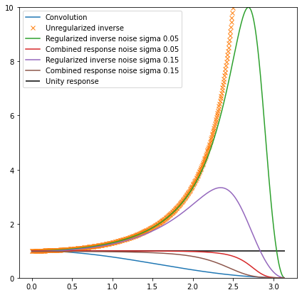
Notice how the inverse response is the same at the beginning of the curve with and without the regularization, but changes dramatically as the convolution attenuates more and more the highest frequencies. It goes to just zero at the Nyquist frequency – as we don’t have any information left there and it not just doesn’t amplify, but also removes noisy signal there. This can be thought of as actual combined deconvolution and denoising!
Here are two examples of the different noise levels and different deconvolution results:
Top: Less noise. Bottom: More noise.
Worth noting how deconvolved results are still noisy, and still not perfectly reconstructing the original image – Wiener deconvolution can give optimal results in the least squares sense (though we simplified it as compared to original Wiener deconvolution and don’t take signal strength into account), but it doesn’t mean it will be optimal perceptually – it doesn’t “understand” our concepts of noise or blur. And it doesn’t adapt in any way to structures present in data…
Deconvolution in practice
We went through the theory of deconvolution, as well as some practical caveats like regularization against noise, so it’s time to put this into practice. I will start with a more “traditional”, slower method, followed by a simplified one, designed for real time and/or GPU applications.
Deconvolution by filter design
The first way of deconvolving is as easy as it gets; use a signal processing package to optimize a linear-phase FIR filter for the desired response. Writing your own that is optimal in the least-squares sense is maybe a dozen lines of Python code – later in the post we will use for a similar purpose. For this section, I used the excellent scipy.signal package.
convolution_filter = [0.25,0.5,0.25]
freq, response_to_invert = scipy.signal.freqz(convolution_filter)
noise_reg = 0.01
coeffs = 21
deconv_filter = scipy.signal.firls(coeffs , freq/np.pi, np.abs(response_to_invert)/(np.abs(response_to_invert)**2+(noise_reg)**2))
The earlier figures I generated this way:
If you’re curious, those are the plots of the generated filters:
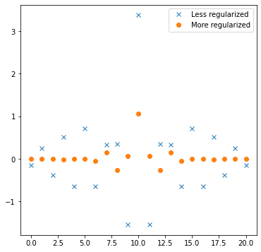
They should match the intuition – a more regularized filter can be significantly smaller in spatial support (doesn’t require “infinite” sampling to reconstruct frequencies closer to Nyquist), and it has less strong gains and less negative weights, preventing oversharpening of the noise. For the stronger filter, we are clearly utilizing all the samples, and most likely a larger filter would work better. Here is a comparison of desired vs actual frequency responses:
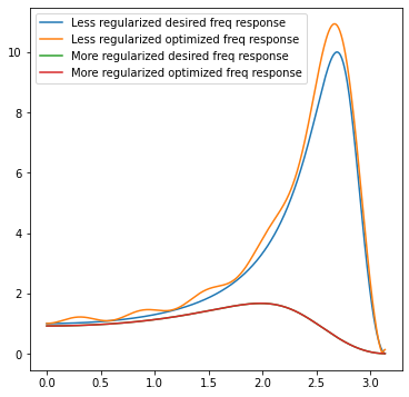
From here, one can go deeper into signal processing theory and practice of filter design – there are different filter design methods, different trade-offs, different results.
But I’d like to offer an alternative method that has a larger error, but is much better suited for real time applications.
Deconvolution by simple filter combination
Finding direct deconvolution filters through filter design works well, but it has one big disadvantage – resulting filters are huge, like 21 taps in the above example.
With separable filtering this might be generally ok – but if one was to implement a non-separable one, using 441 samples is prohibitive. Finding those 21 coefficients is also not instantaneous (require a pseudoinverse of a 21×21 matrix; or in case of non-separable filtering, solving a system involving a 441×441 matrix! Cost can be cut by half or quarter using symmetry of the problem, but it’s still not real-time instantaneous).
In computer graphics and image processing we tend to decompose images to pyramids for faster large spatial support processing. We can use this principle here.
A paper that highly inspired me a while ago was “Convolution Pyramids” – be sure to have a read. But this paper uses a complicated method with a non-linear optimization, which works great for their use-case, but here would be an overkill.
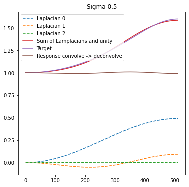
For a simple application like deconvolution, we can use simply a sum of Laplacians resulting from Gaussian filtering instead.
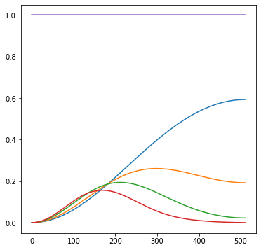
Imagine that we have a bunch of Gaussian filters with sigmas 0.3, 0.6, 0.9, 1.2, 1.5 (chosen arbitrarily) and their Laplacians (difference between levels) plus a “unity” filter that we will keep at 1.0. This way, we have 4 frequency responses to operate with and to try adding to reach the target response:
In numpy, this would be something like this:
def gauss_small_sigma(x: np.ndarray, sigma: float):
  p1 = scipy.special.erf((x-0.5)/sigma*np.sqrt(0.5))
  p2 = scipy.special.erf((x+0.5)/sigma*np.sqrt(0.5))
  f = (p2-p1)/2.0
  return f / np.sum(f)

filters = [gauss_small_sigma(np.arange(-5, 5, 1), s) for s in (0.00001, 0.3, 0.6, 0.9, 1.2, 1.5)]
filters_laps = [np.abs(scipy.signal.freqz(a - b)[1]) for a,b in zip(filters[1:], filters)]
stacked_laps = np.transpose(np.stack(filters_laps))
target_resp = stacked_laps, target - np.ones_like(target)
regularize_lambda = 0.001
solution_coeffs = np.linalg.lstsq(stacked_laps.T.dot(stacked_laps) + regularize_lambda * np.eye(stacked_laps.shape[1]),
                                  stacked_laps.T.dot(target_resp))[0]
Here, solved coefficients are [-17.413, 54.656, -52.741, 20.025] and the resulting fit is very good:
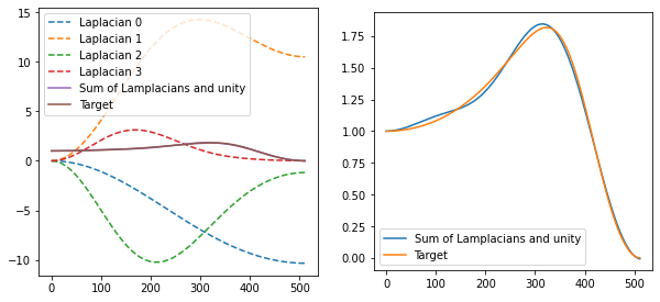
Edit: just right after publishing I realized I missed one Laplacian from plots and the next figure. Off by one error – sorry about that. Hopefully it doesn’t confuse the reader too much.
We can then convert the Laplacian coefficients to Gaussian coefficients if we want. But it’s also interesting to see how contributing Laplacians look like:
As before, the results are not great because we have a relatively large blur and some noise. To improve it for such a combination, we would need to look at some non-linear methods. It’s also interesting that Laplacians seem to be huge in range and value (with my visualization clipping!), but their contributions mostly cancel each other out.
Note that this least squares solve requires operating only on a 5×5 matrix, so it’s super efficient to solve every frame (possibly even per pixel, but I don’t recommend that). It also uses separable, easily optimizable filters.
I chose used blurs arbitrarily, to get some coverage of small sigmas (which can be implemented efficiently). My ex-colleagues had a very interesting piece of work and paper that shows that by iterating the original blur kernel (which can be done efficiently in the case of small blurs; but you pay the extra memory cost for storing the intermediates), you can get a closed form expression coming from a truncated Neumann series. I recommend checking out their work, while I propose a more efficient alternative for small blurs.
Even simpler filter for small blurs
The final trick will come from a practical project that I worked on, and where blurs we were dealing with were smaller in magnitude (sigmas of like 0.3-0.6). We also had a sharpening part of the pipeline with some interesting properties that was authored by my colleague Dillon. I will not dive here into the details of that pipeline.
The thing that I looked at was the use of the kernel used to generate Laplacians – which was extremely efficient on the CPU and DSP and used “famous” dilated a-trous filter. I recommend an older paper that explains well the signal processing “magic” of a repeated comb filtering. Its application for denoising can leave characteristic repeated artifacts due to non-linear blurring, but it’s excellent for generating non-decimating wavelets or Laplacians.
Here is a diagram that +/- explains how it works if you don’t have time to read the referenced paper:
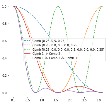
Notice how each next comb filter combined with the previous one approximates full lowpass filter better and better. To get even better results, one would need a better lowpass filter with more than 3 (or 9 in 2D) taps. Those 3 comb filters form also 3 Laplacians (unity vs Comb1, Comb 1 vs combined Comb 1 and 2, combined Comb 2 and 3 vs combined Comb 1 and 2).
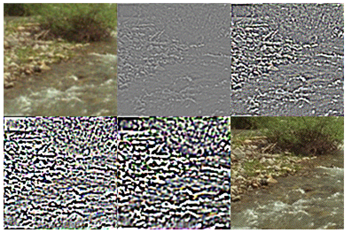
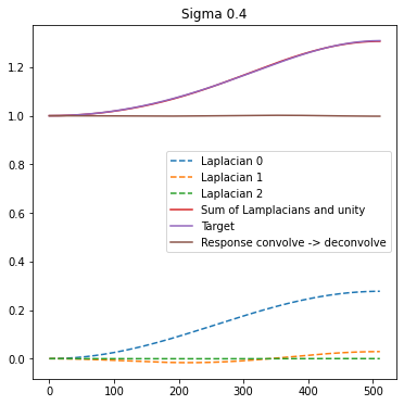
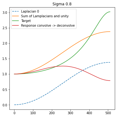
I looked at using those to approximate small sigma deconvolution and for those small sigmas they fit perfectly:
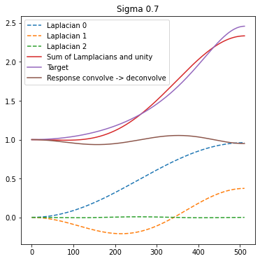
How well does it work in practice on images? Very well!
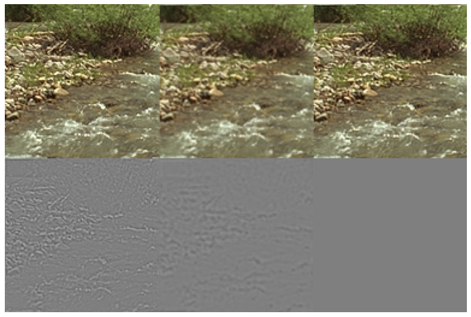
Bottom row: Contributing Laplacian enhancements.
This is for a larger sigma of 0.7. Note also the third coefficient is always close to 0.0, so we can actually use only 2 comb filters and have just 2 Laplacians.
This can be implemented extremely efficiently (two passes of 9 taps; or 4 passes of 3 taps!), requires inverting just a 2×2 matrix (closed formula) and this one could be done per pixel in a shader. My colleague Pascal suggested solving this over a quadrature instead of uniformly sampling the frequency response and even the Gramm matrix accumulation can be accelerated by an order or two of magnitude with not much loss of the fit fidelity.
Bonus – convolution in relationship to sharpening
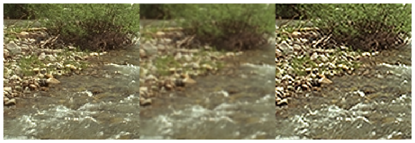
As a small bonus, an extreme case – how well can a silly and simple unsharp mask (yes, that thing where you just subtract a blurred version of the image and multiply it and add back) approximate deconvolution..?
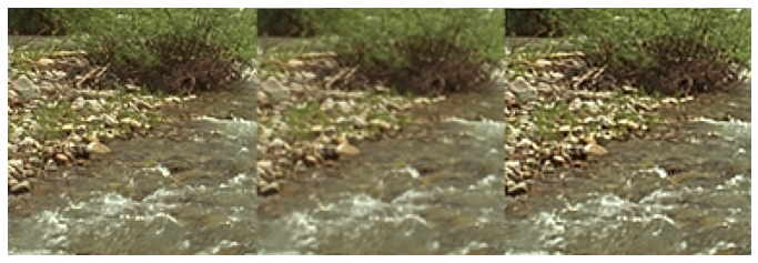
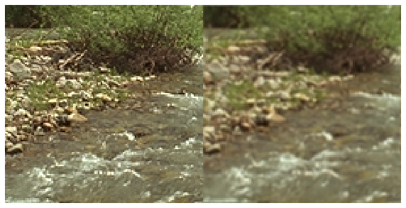
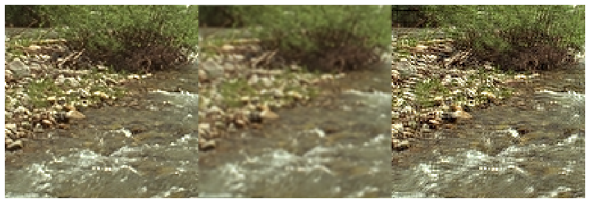
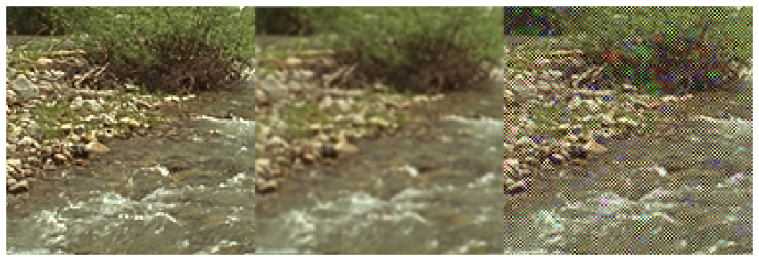
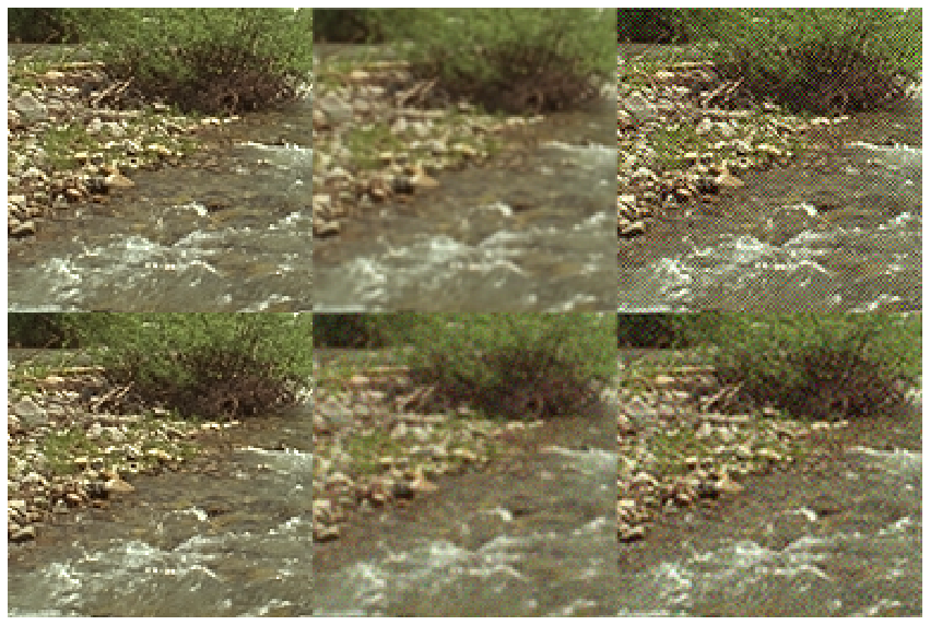
Left: Original image. Center: Blurred through convolution. Right: Unsharp mask deconvolution of a blurry and noisy image
There’s definitely some oversharpening and “fat edges”, but given an arbitrary, relatively large kernel and just a single operation it’s not too bad! For smaller sigmas it works even better. “Sharpening” is a reasonable approximation of mild deconvolution. I am always amazed how well some artists’ and photographers’ tricks work and have a relationship to more “principled” approaches.
Limitations of linear deconvolution and conclusions
My post described the most rudimentary basis of single image deconvolution – its theory, algebraic and frequency domain take on the problem, practical problems, and how to create filters for linear deconvolution.
The quality of linear filters deconvolving noisy signals is not great – still pretty noisy, while leaving images blurry. To address this, one needs to involve non-linearity – local data dependence in the deconvolution process.
Historically many algorithms used optimization / iteration combined with priors. One of the simplest and oldest algorithms worth checking out is Richardson-Lucy deconvolution (pretty good intro and derivation, matlab results), though I would definitely not use it in practice.
Large chunk of work in the 90s and 00s used iterative optimization with image space priors like total variation prior or sparsity prior. Those took minutes to process, produced characteristic flat textures, but also super clean and sharp edges and improved text legibility a lot – and not surprisingly, were used in forensics and scientific or medical imaging. And as always, multi-frame methods that have significantly more information captured over time worked even better – see this work from one of my ex-colleagues, which was later used in commercial video editing products.
Modern way to approach it in a single-frame (but also increasingly more for videos) setting is unsurprisingly through neural networks which are both faster, as well as give higher quality results than optimization based methods.
In my recent tech report I proposed to combine super small and cheap neural networks with “traditional” methods (NN operates at lower resolution and predicts kernel parameters for a non-ML algorithm) and got some decent results:

Any decent nonlinear deconvolution would detect and adapt to local features like edges or textures, and treat them differently from flat areas, trying to amplify blurred local structure, while ignoring the noise. This is a very fun topic, especially when reading about combinations of deconvolution and denoising, very often encountered in scientific and medical imaging, where one physically cannot acquire better data due to physical limitations, costs, or for example to avoid exposing patients to radiation or inconvenience.
Hope you enjoyed my post, it inspired you to look more at the area of deconvolution, and that it demystified some of the “deblurring”, “sharpening”, and “super-resolution” circle of confusion. 🙂

So what tool I can use to make this “deconvolution”
This is a mathematical and image processing formulation of the problem. If you understand blur in your system, you can use Python for modeling and undoing it. Or if you’re not an engineer you can use commercial software that does it (Photoshop has lens blur removal tool I believe).
I would like to recommend a paper that proposes prefilters for sharpness by View Distance and display dpi.
Presentation: https://www.youtube.com/watch?v=D0EcX0NtpW0
Paper: https://diglib.eg.org/handle/10.1111/cgf13942
ABSTRACT
“In this paper we use a simplified model of the human visual system to explain why humans tend do prefer ”sharpened” digital images. From this model we then derive a family of image prefilters specifically adapted to viewing conditions and user preference, allowing for the trade-off between ringing and aliasing while maximizing image sharpness. We discuss how our filters can be applied in a variety of situations ranging from Monte Carlo rendering to image downscaling, and we show how they consistently give sharper results while having an efficient implementation and ease of use (there are no free parameters that require manual tuning). We demonstrate the effectiveness of our simple sharp prefilters through a user study that indicates a clear preference to our approach compared to the state-of-the-art. “
I read this paper and liked the part on sharpening for human “reconstructing filter” a lot! It’s a pity that the theory of generalized sampling is so opaque and theory heavy – I have to admit I don’t fully understand this framework. Need to read it a few more times I think.
Pingback: Gradient-descent optimized recursive filters for deconvolution / deblurring | Bart Wronski