Intro

In this blog post I am going to describe an alternative tool for the graphics and image processing programmers’ toolbox – guided filtering.

Guided filtering is a really handy tool that I learned about from my coworkers, and I was surprised that it is not more popular, especially for real time applications.

As in many – if not most – of my blog posts, I am not going to describe original research of mine, but try to educate, explain some ideas conceived and published by others, focusing on practical application, their pros and cons – and hopefully inspire others.

Given the recent advances in real time rendering, and popularity of “stochastic” techniques – both screen-space (SSAO, screen-space reflections), as well as world-space like ray tracing, there will be more need for efficient, robust, detail preserving denoising of different image signal components.  Most commonly used (joint) bilateral filter is just one of them, but there are some as fast (if not faster!) alternatives and I am going to describe one of them.

This blog post comes with code in form of Google Colab and Python / numpy implementation. I find it really useful that anyone can just run it in their browser, start modifying it and playing with it. Highly recommend it over lonely repos that might not even compile! 🙂

Problem statement

I am going to use here a problem of screen-space ambient occlusion. It is an approximation of some of global illumination effects (visibility, shadowing of indirect illumination) using screen-space depth information. I will not go deeply into how it is computed (I have mentioned a robust, fast and simple technique in an older blog post of mine in the context of temporal techniques), but to meet performance constraints, this technique is computed:

• Usually at lower resolution,
• Using randomized, stochastic sampling patterns, producing noisy results.

Here is an example of raw, unfiltered SSAO output on a Crytek Sponza scene:

Because of small sample count, the results are very noisy, and there are only a few discrete levels of signal (color banding). This image is also half resolution (quarter pixels) as compared to the full image.

We could just blur it to get rid of the noise with a Gaussian filter, but the effect would be… well, blurry:

The main problem with this blurriness – apart from loss of any kind of details – is that it doesn’t preserve the original geometric edges, and when applied to a real scene, would creating halos.

The most common solution to it is joint bilateral filtering.

(Joint) bilateral filter

Bilateral filter is image filter that varies sample weights not only based on image-space distance in pixels, but also the similarity between color samples.

In an equation form this could be written as:

y = Sum(w(x, xij) * xij) / Sum(w(x, xij)
w(x, xij) = wx(i,j) * wy(x, xij)

Where wx is spatial weight, and wy is signal similarity weight. Similarity weight can be any kind of kernel, but in practice the most commonly used one is Gaussian exp(-1/sigma^2*distance^2). Note the sigma parameter here – it is something that needs to be provided by the user – or generally tuned.

Bilateral filters are one of the cornerstones of image processing techniques, providing basis for denoising, detail enhancement, tonemapping etc.

Joint bilateral filter is a form of bilateral filter that uses one signal to create weights for filtering of another signal.

It can be used anytime when we have some robust, noise-free signal along the unreliable, noisy one and we expect them to be at least partially correlated. Example and one of the earliest applications is would be denoising low light images using a second picture of the same scene, taken with a flash.

Joint bilateral filtering can be written in an equation form as:

w(x, xij) = wx(i,j) * wy(z, zij)

Note that here the similarity weight ignores the filtered signal x, and uses a different signal z. I will call this signal a guide signal / guide image – even outside of the context of guided filtering.

In the case of SSAO, we can simply use the scene linear depth (distance of a rendered pixel from the camera plane).

It is most commonly used because it comes for “free” in a modern renderer, is noise-free, clearly separates different objects, doesn’t contain details (like textures) that we wouldn’t want to correlate with the filtered signal – is piece-wise linear.

On the other hand, nothing really prevents us from using any other guide signal / information – like albedo, lighting color, geometric normals etc. Using geometric or detail normals is very often used for filtering of the screen space reflections – as reflections are surface orientation dependent and we wouldn’t want to blur different reflected objects. But in this post I will focus on the simplest case and keep using just the depth.

Let’s have a look at simple joint bilateral filter using depth:

Clearly, this is so much better! All the sharp edges are preserved, and the efficacy of denoising seems quite similar.

Bilateral upsampling

Ok, so we got the half resolution signal quite nicely filtered. But it is half resolution… If we just bilinearly upsample it, the image will just become blurrier.

If we zoom in, we can see it in more details:

Left: 2x point upsampling, Right: 2x bilinear upsampling.

In practice, this results in ugly half-res edges and artifacts and small dark/bright jaggy aliased “halos” around objects.

Luckily, the joint bilateral filtering framework provides us with one solution to this problem.

Remember how joint bilateral filter takes data term into account when computing the weights? We can do exactly the same for the upsampling. (edit: a second publication also from Microsoft research covered this idea the same year!) 

When upsampling the image, multiply the spatial interpolation weights by data similarity term (between low resolution guide image and the high resolution guide image), renormalize them, and add weighted contributions.

This results in much better image sharpness, edge preservation and other than the computational cost, there are no reasons to not do it.

Left: 2x point upsampling, Middle: 2x bilinear upsampling, Right: 2x joint bilateral upsampling.

I highly recommend this presentation about how to make it practical for things like SSAO, but also other applications that don’t require any bilateral denoising/smoothing, like particle and transparency rendering.

As a side note – performing such bilateral upscaling N times – if we have N different effects applied in different places – might be costly at full resolution. But you can use the bilinear sampler and precompute UV offsets once, ahead of time to approximate bilateral upsampling. I mentioned this idea in an older blog post of mine.

To summarize the described workflow so far:

1. Create a low resolution representation of some “robust” signal like depth.
2. Compute low resolution representation of a noisy signal.
3. Perform joint bilateral filtering passes between the noisy signal and the clean low resolution signal.
4. Use a low and high resolution representation of the clean signal for joint bilateral upsampling.

In theory, we could do joint bilateral filtering of the low resolution signal directly at higher resolution, but in practice it is not very common – mostly because of the performance cost and option to use separable filtering directly in lower resolution.

Problems with bilateral filtering

Let me get this straight – bilateral filtering is great, works robustly, and it is the recommended approach for many problems. 

But at the same time, as every technique it comes with some shortcomings and it is worth considering alternatives, so I am going to list some problems.

Lack of separability

One of the caveats of the bilateral filter is that following its definition, it is clearly not separable – as weights of each filter sample, even off the x and y axis depend on the similarity with the filter center.

Unlike Gaussian, a pass over x dimension followed by a pass over the y dimension (to reduce the number of samples from N^2 to N) is not mathematically equivalent… but in practice this is what we do most of the time in real time graphics.

The results are almost indistinguishable:

As expected, there have to be some artifacts:

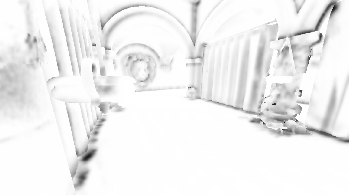
Left: Full NxN bilateral filter. Right: Separable N+N bilateral filter.

Notice the banding on the top of the image, as well as streaks around the lion’s head.

Still, it’s significantly faster and in practice the presence of artifacts is not considered a showstopper. 

I will just briefly mention an alternative to slightly reduce those artifacts – to run the separable filter N times – so iterating over the image x, y, x, y etc. But below is a diagram of clean signal pattern where it will not work / improve things anyway.

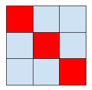
Example pattern of clean signal that separable joint bilateral filtering will ignore completely. Neither horizontal, nor vertical pass can “see” the elements on the diagonal, while a non-separable version would read them directly.

Edit after a comment: Please note that there are many other different ways of accelerating the bilateral filter. They usually involve subsampling in space, either in one sparse pass, or in multiple progressively more dilated ones.

Tuning sensitivity / scale dependence

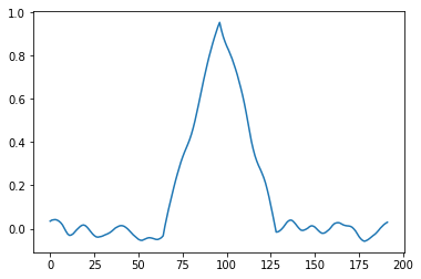
Bilateral filtering has a necessary tuning parameter “sigma”. This makes it inherently scale dependent. Areas where guide signal difference is multiple sigmas won’t get almost any smoothing, while the areas with larger difference will get over-smoothed. I will show this problem with an example of 1D signal.

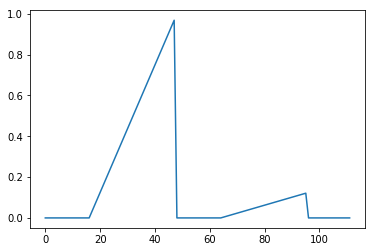
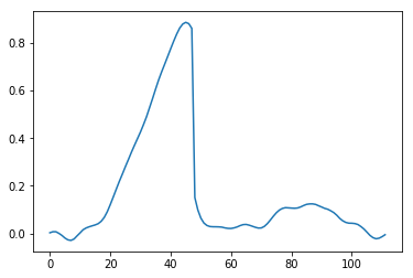
Top: clean 1D guide signal, Bottom: Noisy 1D signal to filter.

We need to pick some sigma, and because of the signal variations here, no choice is going to be perfect. Too large sigma is going to cause over-blurring of the small signal (and rounding of the corners), while too small sigma will under-filter some areas.

Top: Too small sigma causes under-filtering of the signal and some staircase/gradient reversal artifacts, bottom: too large sigma over-blurs the corners, and over-smooths the smaller scale details.

Staircase / piecewise constant behavior / splotches

While bilateral filtering behaves perfectly when the guide/clean signal is piece-wise constant, it can produce undesired look when the clean signal is a gradient / linear ramp – or generally piece-wise linear. In such case it will either produce piece-wise-constant look (very often referred to “cartoony”), gradient reversals, or staircase type of artifacts.

Top: clean signal, middle: noisy signal, bottom: joint bilateral filtered signal – notice some local gradient reversals / staircase artifacts.

Performance cost

Finally, the bilateral filter is not that cheap. Each sample weight requires computation of the kernel function (most often exponential), and there is a need for normalization at the end.

Doing bilateral denoising then followed by bilateral upsampling while saves some computations by doing most of the wide-radius filtering work in low resolution, but still shows some redundancy as well – in the end we are computing bilateral weights and renormalizing twice.

Guided filter – local linear models

Some of those shortcomings are solved by the guided filter. While I as always recommend the original paper – and its idea is brilliant, I had some trouble parsing it (IMO the follow-up, fast guided filter is easier to understand), so will describe it with my own words. 

The main idea is simple: given some local samples, find a best-fit linear relationship between the guide and filtered signal. “Best-fit” is vague, so we will use the linear least squares method – both because it has the optimal behavior (maximum likelihood estimator) in the case of normally distributed data, but also because of it having a simple, closed form and computational efficiency.

This is effectively solving a linear regression problem “what is the linear equation that describes relationship in the data with the smallest squared error”.

Before delving into how to do it, let’s have a look at a few examples of why it might be a good idea. If there is no local variation of the guide signal, linear model will revert to just averaging – so will work correctly in the case of the piece-wise constant signals.

At the same time, one of the main and immediate motivations is that such method will perform perfectly in the case of piece-wise linear signal (as opposed to piece-wise constant of the bilateral filter). So in the case of SSAO – it should give better results anytime you have a depth gradient correlated with change in the filtered signal intensity. 

Similarly, it is in a way a machine learning technique and it should discover linear relationships no matter what is the scale of them – it will automatically infer the scaling parameter from the data.

Let’s see it on the two examples from the previous section – shortcomings of the bilateral filter.

Top: noisy signal, middle: joint bilateral filtered signal – notice some local gradient reversals / staircase artifacts, bottom: same signal filtered with a guided filter. Notice the lack of problematic artifacts.

Top: Bilateral filter with too small sigma, middle: bilateral filter with too large sigma, bottom: parameter-free guided filter.

“There is no such thing as a free lunch”, so there are some shortcomings, but I will cover them in a later section. Now, knowing the motivation behind the local linear regression, let’s have a look at how we can do it.

How to compute linear regression efficiently

How to solve linear least squares is one of the most common entry-level position machine learning interview questions. This is so widely described topic that it doesn’t make sense for me to rederive here the normal equations (Inverse(X*X^T)*X^T*b) using the matrix notation form. Instead, I will just point out to the univariate linear regression wikipedia article, that shows how to solve it easily with simple terms like covariance, variance, and mean.

The beauty of it is that you can do it just by accumulating raw (not even centered!) moments. This is not the most numerically robust way to do it, but it is extremely efficient. In pseudo-code, it would be something like:

X = Sum(x)

Y = Sum(y)

X2 = Sum(x*x)

XY = Sum(x*y)

A = (XY - X * Y) / (X2-X*X + reg_constant)

B = Y - beta * X

This is so simple and beautiful – we are looking at just sums, fused multiply-adds and a single division! The sums are not only completely separable, but also can be computed very efficiently using SAT/integral images.

We can also do a weighted linear least squares – and just multiply the moments by weights when accumulating them. I will use Gaussian weights in my examples due to reverting to pleasantly-looking (and not very alias prone) Gaussian filter in the case of constant signals.

Note the reg_constant here. In practice for perfectly flat signals you have to add some regularization to avoid divisions by zero or NaNs (or simply answering an ill-posed question “what is the linear relationship between a signal that doesn’t change at all and a different one?”). Such Tikhonov regularization can also make the model “smoother” and reverting more and more to local mean (like regular smoothing). You can observe the effect in the following animation – as regularization increases, the result looks more and more like a simply blurred signal.

If you use a separable kernel like Gaussian for weighting of the accumulated moments, this means that it can still be done in a separable way. While storing 4 values from 2 signals might seem sub-optimal and increase the memory bandwidth usage (especially those moments as squared variables are precision-hungry…) or the register pressure, total linearity of moment accumulation is suitable for optimizations like using local / group shared memory/cache and avoiding going back to the main memory completely. It can be done pretty efficiently with compute shaders / OpenCL / CUDA.

Results

How does it work in practice? Here is the result of filtering of our sponza SSAO:

And by comparison again bilateral filter:

The results are pretty similar! But there are some subtle (and less subtle) differences – both solutions having their quality pros and cons. 

For better illustration, I include also a version that toggles back and forth between them. Guided filter is the slightly smoother one.

I will describe pros and cons later, but for now let’s have a look at another pretty cool advantage of local linear models.

Upsampling linear models

After we have done all the computations of finding a local linear regression model that describes the relationship between the filtered and guide signal, we can use this model at any scale / resolution.

We can simply interpolate the model coefficients, and apply to a higher (or even lower) resolution clean / guide signal. It can be used to greatly accelerate the image filtering.

This way, there is no need for any additional bilateral upsampling.

In full resolution, just fetch the interpolated model coefficients – like using hardware bilinear sampling – and apply them with a single fused multiply-add operation. Really fast and simple. The quality and the results achieved such way are excellent.

Top: Joint bilateral upsampling of guide filtered image, bottom: bilinearly interpolated local linear model.

While those results are very similar, there are two quality advantages of the linear model upsampling – it can at the same time preserve some details better than joint bilateral upsampling, as well as produce less bilinear artifacts. Both of them come from the fact that it is parameter-free, and discovers the (linear) relationships automatically.

Left: joint bilateral upsampling of the results of the guided filter, right: upsampling of the local linear model coefficients. Notice that both the details are sharper, as well as have less of bilinear artifacts.

On the other hand, in this case there are two tiny 2 pixel-wide artifacts introduced by it – look closely at the right side of the image, curtains and a pillar. What can cause such artifacts? If the low resolution representation lacks some of the values (e.g. a single pixel hole), linear model that is fitted over a smaller range and then extrapolated to those values will most likely be wrong…

The linear model upsampling is so powerful that it can lead to many more optimizations of image processing. This post is already very long, so I am only going to reference here two papers (one and two) that cover it well and hopefully will inspire you to experiment with this idea.

Pros and cons

Pro – amazingly simple and efficient to compute

Pretty self-explanatory. In the case of two variables (input-output), local linear regression is trivial to compute, uses only the most basic operations – multiply-adds and can be used with separable convolutions / summations or even SATs.

Pro – works at multiple image scales

The second pro is that local linear regression almost immediately extends to multi-resolution processing with almost arbitrary scaling factor. I have seen it successfully used by my colleagues with resolution compression factors higher than 2x, e.g. 4x or even 8x.

Pro – better detail preservation at small detail scales

Local linear models are relatively parameter-free, and therefore can discover (linear) relationships no matter the guide signal scale. 

Here is an example of this effect:

Left: joint bilateral filter, right: guided filter. 

Notice not only much cleaner image, but better preservation of AO that increases with depth around the top right of the image. Joint bilateral filter is unable to discover and “learn” such relationship. On the other hand, details are gone around the left-bottom part of the image, and I will explain the reason why in a below section called “smudging”.

Pro – no piecewise constant artifacts

I have mentioned it before, but piecewise constant behavior, “chunkiness”, gradient reversal etc. are all quite objectionable perceptual effects of the bilateral filter. Local linear regression fixes those – resulting in a more natural, less processed looking image.

Pro or con – smoother results

Before going into the elephant in the room of over blurring and smudging (covered in the next point), even correct and well behaved local linear models can produce smoother results.

Here is an example:

Left: joint bilateral filter, right: guided filter without any regularization.

Notice how it can be both great (shadow underneath the curtain), as well as bad – overblurred curtain shape.

Why does such oversmoothing happen? Let’s look at a different part of the image.

I have marked with a red line a line along which the depth increases just linearly. Along this line, our signal goes up, and down in oscillatory patterns. What happens if we try to fit a single line to something like this? The answer is simple – oscillations along this line will be treated as noise and smoothed no linear relationship will be discovered, so the linear model will revert to local mean.

Con – “smudging”

This is what I personally find the biggest problem with the guided filter / local linear models and limitation of a linear-only relationship. Notice the blurry kind of halo around here:

Left: joint bilateral filter, right: guided filter.

Why is it happening only around those areas? I think about it this way – a significant discontinuity of signal and a large difference “dominates” the small-scale linear relationships around it.

I have compared here two signals:

Left: flat signal followed by a small signal variation can be fit properly when there are no discontinuities or conflicting gradients, right: presence of signal discontinuity causes the line fitting to completely ignore the small “ramp” on the right.

Overall this is a problem as human visual system is very sensitive to any kind of discontinuities and details suddenly disappearing around objects look like very visible halos…

This reminds me of the variance shadow mapping halos/leaking.

Would fitting a second order polynomial, so tiny parabolas help here (another shadow mapping analogy – like in moment shadow mapping)? The answer is yes! It is beyond the scope of this blog post, but if you are interested in this extension, be sure to read till the last section of this blog post. 🙂  

Con – potential to create artifacts

I have mentioned above that using bilateral upsampling can cause some artifacts like:

Those are less common and way less objectionable than jagged edges and broken-looking bilinear interpolation, but getting rid of those might be very hard without either too strong / too over-smoothing regularization, or some tricks that go well beyond the scope of a simple linear regression (additional data weighting, input clamping, stochastization of the input etc.).

Con – regression of multiple variables more costly

Unlike the joint bilateral filter where weight is computed once for all of the channels, if you want to filter an N channel signal using a single channel guide, the computation and storage cost goes up N times! This is because we have to find local linear model that describes the relationship between the guide signal and each of the channels separately… In the case of RGB images this might be still practical and acceptable (probably not for multi-spectral imaging though 🙂 ), but it might be better to do it only on e.g. luma and upsample and process the chroma with some different technique(s)…

Con – memory requirements

The local storage memory costs of regression are at least twice as large as the bilateral filter for the number of channels. Unfortunately, those are also “hungry” for precision (because of using squared raw moments) and you might have to use twice more bit depth than for your normal filtered and guide signals.

Extending it and taking it further

I hope that after this post I have left you inspired to try – and experiment with – a slightly different tool for various different image processing operations – filtering, denoising, upsampling, mixed resolution processing. It is trivial to prototype and play with, but it goes beyond simple linear correlation of two variables. 

In fact, one can extend it and use: 

• Any order polynomial least squares regression, including modelling of quadratic, cubic, or any higher order functions,
• Multivariate modelling, including regression of the output from multiple guide signals.

Both of those require going back to the least squares framework, solving the normal equations, but can still be solved via accumulation of RAW moments of those signals to construct a larger covariance matrix.

Here is a quick, animated comparison in which I added depth squared for the regression.

A sequence of joint bilateral filter, first, and the second order least squares regression. Second order linear regression (parabola fitting) improves the results quite drastically… but obviously at additional performance cost (7 moments accumulated instead of 4) and some more noise preservation.

Using more input signals comes with an additional cost, but does it always guarantee increased quality? There are two answers to this question. First one – “kind of”, as if there was no linear relationship with this additional variable and no correlation, it should be simply ignored. The second one is “yeah in terms of absolute error, but kind of not, when it comes to perceptual error”.

The problem is that more complex models can “overfit”. This is known in ML as bias-variance trade-off and more variance = more noise remaining after the filtering. We can see it in my toy example – there is clearly somewhat more noise on the left column.

As an example of a paper that uses multivariate regression, is this recent work from Siggraph 2019. It is work solving directly the problem of rendering denoising, and they use multiple input signals like normals, world space positions, world space positions squared etc. They use a lot of tricks to make linear models work over non-overlapping tiles (sparse linear models) – I personally found it very inspiring and highly recommend it!

I will conclude my post here, thanks for reading such a long post – and happy adventures in image filtering!

PS. Be sure to check out and play with Colab code that comes with this blog post.

References

Scalable Ambient Obscurance, Morgan McGuire, Michael Mara, David Luebke

Flash Photography Enhancement via Intrinsic Relighting, Elmar Eisemann, Freedo Durand

Joint Bilateral Upsampling, Johannes Kopf, Michael F. Cohen, Dani Lischinski, Matt Uyttendaele

Image-Based Proxy Accumulation for Real-Time Soft Global Illumination, Peter-Pike Sloan, Naga K. Govindaraju, Derek Nowrouzezahrai, John Snyder

Mixed Resolution Rendering in Skylanders: Superchargers, Padraic Hennessy 

A Low-Memory, Straightforward and Fast Bilateral Filter Through Subsampling in Spatial Domain, Francesco Banterle, Massimiliano Corsini, Paolo Cignoni, Roberto Scopigno

Edge-Avoiding À-Trous Wavelet Transform for fast Global Illumination Filtering, Holger Dammertz, Daniel Sewtz, Johannes Hanika, Hendrik P.A. Lensch

Guided Image Filtering, Kaiming He

Fast Guided Filter, Kaiming He, Jian Sun

Deep Bilateral Learning, Michaël Gharbi, Jiawen Chen, Jonathan T. Barron, Samuel W. Hasinoff, Frédo Durand

Bilateral Guided Upsampling, Jiawen Chen, Andrew Adams, Neal Wadhwa, Samuel W. Hasinoff

Variance Shadow Maps, William Donnelly, Andrew Lauritzen

Moment Shadow Mapping, Christoph Peters, Reinhard Klein 

Blockwise Multi-Order Feature Regression for Real-Time Path Tracing Reconstruction, Koskela M., Immonen K., Mäkitalo M., Foi A., Viitanen T., Jääskeläinen P., Kultala H., and Takala J.