Introduction

In this blog post, I am going to continue exploration of compressing whole PBR texture sets together (as opposed to compressing each texture from the set separately) and using the fact that those textures are strongly correlated.

In my previous post, I have described how we can “decorrelate” some of the channels using PCA/SVD and how many of the dimensions in such a decorrelated space contain small amount of information, and therefore can be either dropped completely, stored at a lower resolution, or quantized aggressively. This idea is a backbone of almost all successful image compression algorithms – from JPEG to BC/DXT.

This time we will look at exploring some redundancy across both the stored dimensions, as well as the image space using sparse methods and kSVD algorithm (original paper link).

From my personal motivation, I wanted to learn more about those sparse methods, play with implementing them and build some intuition – one of my coworkers and collaborators on my previous team at Google, Michael Elad is one of the key researchers in the field and his presentations inspired and interested me a lot – and as I believe that until you can implement and explain something yourself, you don’t really understand it – I wanted to explore this fascinating field (in a basic, limited form) myself.

First I am going to do present a simplified and intuitive explanation of what “sparsity” and “overcompletness” mean and how their redundancy can be an advantage. Then I will describe how we can use sparse approximation methods for tasks like denoising, super-resolution, and texture compression. Then I will provide a quick explanation of k-SVD algorithm steps and how it works, and finally show some results / evaluation for the task of compressing PBR material texture sets.

This post will come with a colab notebook (soon – I need to clean it up slightly) so you can reproduce all the code and explore those methods yourself.

Sparse and dictionary based methods in real-time rendering?

I tried to look for some other references to dictionary based methods in real time rendering and was able to find only of three resources: a presentation by Manny Ko and Robin Green about kSVD and OMP, a presentation by Manny Ko about Dictionary Learning in Games, and a mention of using Vector Quantization for shadow mask compression by Bo Li. VQ is a method that is more similar to palletizing than full dictionary learning, but still a part of the family of sparse methods. I recommend those presentations, (a lot of what I describe about the theoretical part – and how I describe – overlaps with them) and if you are aware of any more mentions of those IMO underutilized methods in such a context, please leave a comment and I’ll be happy to link.

Vector storage – complete and orthogonal basis, vs overcomplete and sparsely used frames / dictionaries

To explain what are sparse methods, let’s start with a simple, 2 dimensional vector. How can we represent such a vector? “This is obvious, we can just use 2 numbers, x and y!”. Sure, but what do those numbers mean? They correspond to an orthonormal vector basis. x and y represent actually a proportion of position along the x axis, and the y axis. If you have done computer graphics, you know that you can easily change your basis. For example, a vector can be decribed in so called “world space” (with arbitrary, fixed point), “camera / view space”, or for some simple video game AI purpose in space of a computer-controlled character.

Vector basis might have different properties. Two that are very desired are orthogonality and normality, often combined together as orthonormal basis. Orthonormality gives us trivial way of changing information between two basis back and forth (no matrix inversion required, no scaling/non-unity Jacobians introduced) and some other properties related to closed form products and integrals – it’s beyond scope of this post, but I recommend “Stupid Spherical Harmonics Tricks” from Peter-Pike Sloan for some examples how SH being orthonormal makes it a desired basis for storing spherical signals.

Choice of “the best” basis matters a lot when doing compression – I have described it in my previous blog, but as a quick refresher, “decorrelating” dimensions can give us basis in which information is maximized in each sequential subset of dimensions – meaning that the first dimension has the most information and variability present, the next one the same or smaller amount etc. This is limited to linear relationships and covariance, but lots of real data shows linear redundancy.

One of the requirements of a space to be a basis is completeness and uniqueness of representation. Uniqueness of the representation means that given a fixed basis, there is only a single way to describe a vector in this space. Completeness means that every vector can be represented without loss of information. In my last post, we looked at the truncated SVD – which is not complete, because we lose some original information and there is no way how we can represent it back.

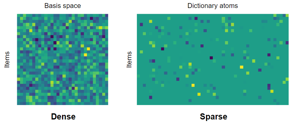
What is quite interesting is that we can go further than vector basis and go towards overcomplete frames (let’s simplify – a lot – for the purpose of this post and say that frame is just “some generalization” of a basis). This means that we have more vectors in space than the “rank” of the information we want to store. Overcomplete frames can’t be orthogonal or unique (I encourage readers for whom this is a new concept to try to prove it – even if just intuitively). Sounds pretty useless for information compression? Not really, let me give here a visual example:

Note that while in the case of overcomplete frame every point can be described in infinitely many ways (just like x + y = 5 has infinitely many solutions of x and y values that satisfy it), we usually are going to look for a sparse representation. We want as many of the components to be zero (or close to zero enough so that we can discard them, accepting some errors), and the input vectors described by a linear combination of less frame vectors than the size of the original basis.

If this description seems vague, looking at the above example – with complete basis, we generally need two numbers to describe the input point set. However, with an overcomplete frame, we can use just a single 2-bit basis index and a float value describing magnitude along it:

Yes, we lose some information, and there is an approximation error – but there is always an error in the case of lossy compression – and the error in such a basis is way smaller than from any truncated SVD (keeping a single dimension of orthogonal basis).

Terminology wise – we commonly refer to a frame vector as atom, and collection of atoms as dictionary – and I will use atoms and dictionary mostly throughout this post.

Also note – we will come back to this later in the next section – I have used here a 2D example and a 1-sparse representation (single atom to represent input) – but with higher dimensions, we can (and in practice do) use multiple atoms per vector – so if you have 16 atoms, any representation that uses 1-15 of them can be considered sparse. Obviously if the input space is 3D, and your dictionary has 20 atoms, while a 10 atom representation of a vector “could” be seen as sparse, it probably won’t make sense for most practical scenarios.

Sparsity and images – palettes and tiles

Now I admit, this 2D case is not super compelling. However, things start to look much more interesting in some much higher dimensions. Imagine that instead of storing 20 numbers for a 20 dimensional vector, you could store just a few indices and a few numbers – in very high dimensions, sparse representations get more and more interesting. Before going towards high dimensional case, let me just show some interesting connection – what happens if for a single pixel of e.g. RGB image we store only index (not even a weight) from a dictionary? Then we end up with an image palette.

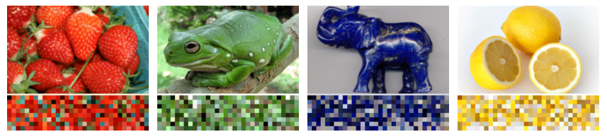
Image palettization is an example of a sparse representation method! One of many algorithms to compute image palette it is k-means, which is a more basic version of k-SVD that I’m going to describe later.

Palettization generalizes to many dimensions – if you have a PBR texture set with 20 channels, you can still palettize it – just your entries will be 20 dimensional vectors.

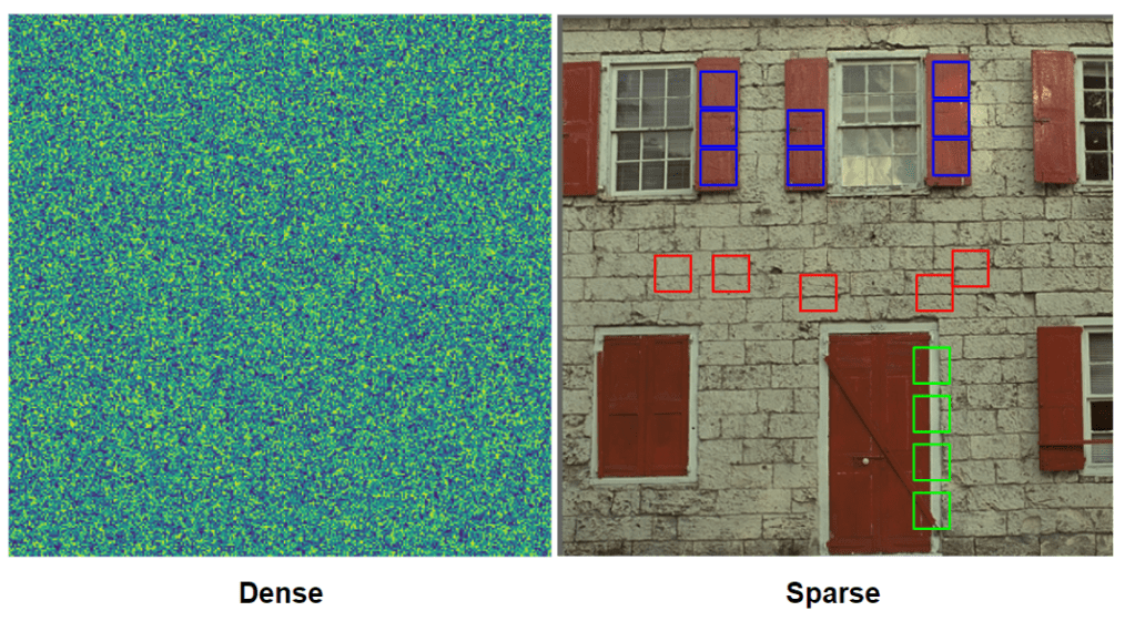
However, we can go much further and increase the dimensionality (hoping for more redundancy in more dimensions) much further. Let’s have a look at this Kodak dataset image and at image tiles:

There is lots of self-similarity in this image – not just within pixel values (those would palettize very well), but among whole image patches! In such a scenario, we can take a whole patch to become our input vector. I have mentioned in the past that thinking beyond “image is 2D matrix / 3D tensor” is one of the most important concepts in numerical methods for image processing, but as a recap, we can take an RGB image and instead of a tensor, represent it by a matrix:

Or we can go even further, and represent it as a single vector:

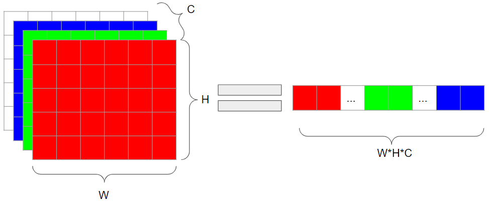
So you can turn a 16×16 RGB tile into a single 768 dimensional vector – and with those 16×16 tiles, a 512 x 512 x3 (RGB) image into a 32×32 image of 768 vectors. This takes time to get used to, but if you internalize this concept (and experiment with it yourself), I promise it will be very useful!

What are sparse methods useful for?

Sparse methods were (and to a lesser extent still are) a “hot” research topic because of a simple “philosophical” observation – the world we live in, and the signals we deal with (audio, images, 3D representation), are in many ways sparse and self-similar.

A 100% random image would not be sparse, but images that we capture with cameras or render are in some domains.

I will not present any proofs of it (also personally I haven’t seen one that would be both rigorous and not handwavy, while staying intuitive), however let me describe some implications and use-cases of it.

Compression

Very straightforward and the use-case I am going to focus on – if instead of storing full “dense” information of a large, multidimensional vector (like image tile), we can instead store a dictionary, and indices of atoms (plus their weights). If the compressed signal was truly sparse in some domain, this can result in massive compression ratios.

Denoising

What happens when we add white noise to a sparse signal? It’s going to become non-sparse! Therefore by finding best possible sparse approximation of it, we are going to effectively decompose it into sparse and non-sparse component, which is going to be discarded and hopefully, corresponds to noise.

Super-resolution

Principle of self-similarity and sparsity can be used for super-resolution of low-resolution, aliased images. Different “phases” of the sampled aliased signal produce different samples, but if we assume there is an underlying common shared representation, we could find it and reconstruct them.

In this example if we correctly located all the aliased tiles and be certain that single, same high resolution atom corresponds to all of them, then we’d have enough information to remove most of the aliasing and reconstruct the high resolution edge.

Computer vision

Computer vision tasks like object recognition or object classification don’t work very well with hugely dimensional data like images. Almost all computer vision algorithms start by constructing some representation of the image tile – corner, line detection. While in the “old times” those features were hard-coded, nowadays state of the art relies on artificial neural networks with convolutional layers – and the convolutional layers with different filter banks jointly learn the dictionary (edges, corners, higher level patterns), as well as use of this dictionary data (I will mention this connection around the end of this post).

Compressive sensing / compressed sensing

This is a really wild, profound idea that I have learned about just this year and definitely would like to explore more. If we assume that the world and signals we sample are sparse in “some” domain and we know it, then we can capture and transmit much less information (orders of magnitude less!), like random subsamples of the signal. Later we can recompute the missing pieces of the information by forcing sparsity of the reconstruction in this other domain (in which we we know the signal is sparse). This is really interesting and wild area – think about all the potential applications in signal/image processing, or in computer graphics (strongly subsampling expensive raytracing or GI and easily reconstructing the full resolution signal).

Note: Sparsity of simple, orthogonal basis

It is important to emphasize that you don’t need any super fancy overcomplete dictionary to observe signal sparsity. Even simple, orthogonal basis can be sparse – for example Fourier transform, DCT, image gradient domain, decimating wavelets – and many of them are actually very good / close to optimal in “general” (average of different possible images) scenarios. This is a base for many other compression algorithms.

kSVD for texture and material compression

Later in this post, I am going to describe the k-SVD algorithm – but first, let’s look at use of sparse, dictionary representations and learning for PBR material compression.

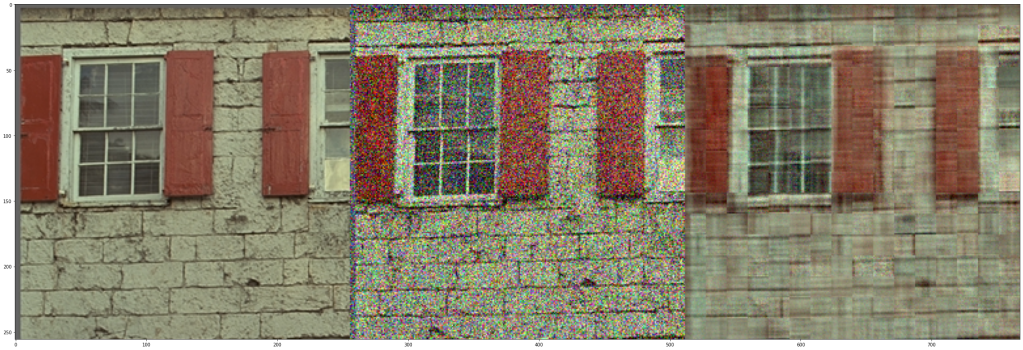
I have stated the problem and proposed a simple solution in my previous blog post. As a recap, PBR materials consist of multiple textures representing different physical properties of a surface of a material. Those properties represent surface interaction with light through BRDF models. Different parts of that texture might correspond to different surface types, but usually large parts of the material correspond to the same surface with the same physical properties. I have demonstrated how those properties are globally correlated. Let’s have a look at it again:

After my longish introduction, it might be already clear that we can see lots of self-similarity in this image and very similar local patches. Maybe you can even imagine how those atoms will look like – “here is an edge”, “here is a stone top”, “here is a surface between the stones” that repeat themselves across the image.

It seems that it should be possible to reuse this “global” information and compress it a lot. And indeed, we can use one of sparse representation learning algorithms, kSVD to both find the dictionary, as well as fit the image tiles to it. I will describe the algorithm itself below, but it was used in following way:

• Split the NxN image into n x n sized tiles after subtracting image mean,
• Set the dictionary size to contain m atom tiles,
• Run kSVD to learn the dictionary and allowing for up to k atoms per tile,
• Recombine the image.

Just for the initial demo (not optimal parameters, I selected the dictionary to contain 8×8 tiles, dictionary sized like 1/32th of the original image, 8 atoms per tile). Afterwards, the texture set will look like this:

I’m presenting it in a low resolution as later I will look more into proper comparisons and the effect of some parameters. From such a first look, I’d say it doesn’t look too bad at all given that per every tile instead of storing 8x8x9 numbers, we store only 9 indices and 9 weights, plus the dictionary is only 1/32th of the orignal image!

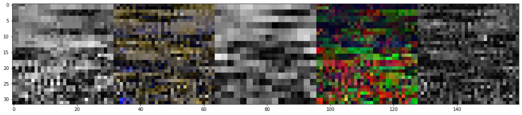
But more importantly, how do the atoms / dictionary look like? Note: atoms are normalized across all channels and we have subtracted the image mean; I am showing absolute value of each pixel of each atom:

Ok, this looks a bit too messy for my taste. Let’s sort them based on similarity (greedy, naive algorithm: start with the first tile, find most similar to it, then proceed to the next tile until you run out of tiles):

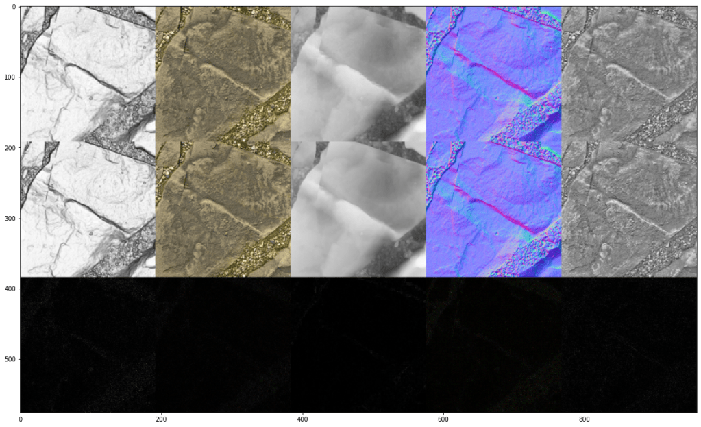
Important note: from the above 5 differently colored subsets, first 8×8 tile of each of them corresponds to the same atom. They are sliced across different PBR properties for visualization purpose only (I don’t know about you, but I don’t like looking at 9 dimensional images😅).

This is hopefully clearer and also shows that there are some clear “categories” of patches and words in our dictionary: some “flat” patches with barely any texture or normal contribution at all, some strong edges, and some high frequency textured regions. An edge patch will show an edge both in normal-map as well as the AO, while a “textured” patch will show texture and variation in all of the channels. Dictionary learning extended correlation between global color channels to correlation of full local structures. I think this is pretty cool and the first time I saw it running I was pretty excited – we can automatically extract quite “meaningful” (even semantically!) information and how the algorithm can find some self-similarities, repeating patterns and use it to compress the image a lot.

I will come back to analyzing the compression and quality (as it depends on the parameters), but let’s now look at how the k-SVD works.

k-SVD algorithm

I have some bad news and some good news. The bad news are that finding optimal dictionary and atom assignments is NP-Hard problem. ☹ We cannot solve it for any real problems in reasonable time. The good news is that there are some approximate/heuristic algorithms that perform well enough for practical applications!

k-SVD is such an algorithm. It is a greedy, iterative, alternating optimization algorithm that is made of the following steps:

1. Initialize some dictionary,
2. Fit atoms to each vector,
3. Update the dictionary given current assignment
4. If satisfied with the results, finish. Otherwise, go back to step 2.

This going between steps 2 and 3 is the “alternating” part, and repeating it is “iterative”.

Note that there are many variations of the algorithm and improvements in many follow-up papers, so I will look at some flavor of it. 🙂 But let’s look at each step.

Dictionary initialization

For the dictionary initialization, you can apply many heuristics. You can start with completely random atoms in your dictionary! Or you can take some random subset of your initial vectors / image tiles. I have not investigated this properly (I am sure there are many great papers on initialization that maximizes the convergence speed), but generally taking some random subset seems to work reasonably. Important note is that you’d want your atoms to be “normalized” across all channels – you’ll see why in the next step.

Atom assignment

For the atom assignment, we’re going to use Orthogonal Matching Pursuit (OMP). This part is “greedy” and not necessarily optimal. We start with the original image tile and call it a “residual”. Then we repeat the following:

1. Find the best matching atom compared to residual. To find this best matching atom according to squared L2 norm, we can simply use dot product. (Think and try to prove why the dot product – cosine similarity of normalized vectors – ordering is equivalent to the squared L2 norm, subject to offset and scale).
2. Looking at all atoms found so far, do a least squares fit against the original vector.
3. Update the residual.

We repeat it as many times as the desired atom count, or alternatively until error / residual is under some threshold.

As I mentioned, this is a greedy and not necessarily optimal part. Why? Look at the following scenario where we have a single 4 dimensional vector, 3 atoms, and allow max 2 atoms per fit:

Given our yellow vector to fit, at the first step if we find the most similar atom, it is going to be the orange one – the error is the smallest. Then we would find the green one, and produce some combination that would produce 2 last dimensions too high/too low – a non-negligible error. By comparison, optimal, non-greedy assignment of 2 atoms “red” and “green” would produce zero error!

Greedy algorithms are often reasonable approximations that run fast enough (the decision made is only locally optimal, so we can consider very small subset of solutions), but in many cases are not optimal.

Dictionary update

In this pass, we assume that our atom assignment is “fixed” and we cannot do anything about it – for now. We go even further, as we look at each atom one by one, and assume that all the other atoms are also fixed! Given almost everything fixed, we optimize: given this assignment and all the other atoms being fixed, what is the optimal value for this atom?

So in this example we will try to optimize the “red box” atom, given two “purple box” items using it.

The way we approach it is solving the following: if there was no this atom contribution, how can we minimize the error of all the atoms using it? We look at all errors of every single item using this atom and try to find some single vector that multiplied by different weights will maximize the removal of average of those errors (so matching it).

In a visual form, it will look something like this:

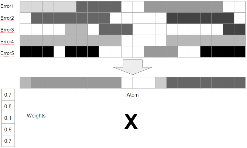
If you are reader of this blog, I hope you recognized that we are looking for a separable, rank 1 approximation of the error matrix! This is where the SVD of k-SVD comes from – we use truncated SVD and compute a rank 1 approximation of the residual. One of separable vectors will be our atom, the other one – updated weights for this atom in each approximated vector.

Note that unlike the previous step, which could lead to unoptimal results, here we have at least a guarantee that each step will improve the average error. It can increase the error of some items, but on average / in total it will always be decreased (or it would have been the same if SVD would found that the initial atom and the weight assignment were already minimizing the residual).

Also note that updating the atoms one by one and updating the weights / residuals at the same time makes it similar to Gauss-Seidel method – resulting in a faster convergence, but at a cost of sacrificed parallelism.

And this is roughly it! We alternate the steps of assigning atoms and updating them until we are happy with the results. There are many nitty-gritty details and follow-up papers, but described like this, kSVD is pretty easy to implement and works pretty well!

How many iterations do you need? This is a good question and probably depends on the problem and those implementation details. For my experiments I was using generally 8-16 iterations.

Different parameters, trade-offs, and results

Note for this section – I am clearly not a compression expert. I am sure there are some compression specific interesting tricks and someone could do a much better analysis – I will not pretend to be competent in those. So please treat it as mostly theoretical analysis from a compression layman.

I will analyze all three main parameters one by one, but first, let’s write down a formula for general compression/storage cost:

Image tiles themselves – k indices, k weights for each of the tiles. Indices need as many bits as log2 of the number of atoms m in the dictionary, and the weights need to be quantized to b bits (which will affect the final precision/error). Then there is the dictionary, which is going to be simply m of n*n sized tiles, each element containing original number of dimensions. So the total storage is going to be:

It’s worth thinking about comparing it to a “break even” ratio, so simply N*N*d. Ignoring the image, dictionary break even is m <= (N/n)^2. Ignoring the dictionary, image break even is:

Seeing those formulas, we can analyze the components one by one.

First of all, we need to make sure that m is small enough so that we actually get any compression (and our dictionary is not simply the input image set 🙂 ). In my experiments I was setting it to 1/32-1/16 of N^2 total tiles of the input for larger tiles, or simply fixed small value for very small tiles.

Then assuming that m * n^2 is small enough, we focus on the image itself. For better compression ratios we would like to have tile size n as large as possible without blowing this earlier constraint – this is a quadratic term. As usually, think about the extreme: a tile 1×1 is the same as no tiling/spatial information at all (still might offer a sparse frame alternative to SVD discussed in my previous post), and large tiles means that our “palette” elements are huge and there are few of them.

Generally, for all the following experiments, I looked only at very significant compression ratios (mentioned dictionary itself being 3-6% size of the input) and visible / relatively large quality loss to be able to compare the error visually.

People more competent in compression will notice lots of opportunities for improvements – like splitting indices from weights, deinterleaving the dictionary atoms, exploiting the uniqueness of atom indices etc. – but again, this is outside of my expertise.

Because of that, I haven’t done any more thorough analysis of the “real” compression ratios, but let’s compare a few results in terms of image quality – both subjective, and objective numbers.

Tile size 1, 3 atoms per pixel, dictionary 32 atoms -> PSNR 34.9

This use-case is the simplest, as it is a sparse equivalent of the SVD we have analyzed in my previous post. Instead of dense 6 weights per pixel (to represent 9 features), we can get away with just 3 and just 32 elements in the dictionary, we can a pretty good SNR! Note however the problem (will be visible on those small crops in all of our examples) – tiny green grass islands disappear, as they occupy tiny portion of the data and don’t contribute too much to the error. This is also visible in the dictionary – none of the elements is green. Apart from it, the compressed image looks almost flawless.

Tile size 2, 4 atoms per tile, dictionary 256 atoms -> PSNR 32.16

In this case, we switch to a tiled approach – but with tiny, 2×2 tiles. We have as many weights per tile, as there are pixels per tile – but pixels were originally 8 channel and now we have per atom only a single weight. The PSNR / error are still ok, however the heightmap starts to show some “chunkiness”. In the dictionary, we can slowly start to recognize some patterns – and how some tiles represent only low frequency, while other higher frequency patterns! The exception is the heightmap – it wasn’t correlated too much with the other channels details, which explains errors and lack of high frequency information. A larger dictionary or more atoms per tile would help to decorrelate those.

Tile size 4, 8 atoms per tile, 6% of the image in dictionary -> PSNR 32.76

4×4 tiles is an interesting switching point as we can compress dictionary with the hardware BC compression. We’d definitely want that, as the dictionary gets large! Note that we get less atoms per tile than there were pixels in the first place! So it’s not only compressing the channel count, but also less than actual pixel count. The dictionary looks much more interesting – all those tiny lines, edges, textured areas.

Tile size 8, 12 atoms per tile, 6% of the image in dictionary -> PSNR 28.11

At this point, the compression got very aggressive (per each 8×8 pixels of the image, we store only 12 weights and indices, that both can be quantized!) – and the tiles are the same size as JPG ones. Still, visually looks pretty good, and the oversmoothing of normals shouldn’t be an issue in practice – but if you look very closely at the height map, you will notice some blocky artifacts. The dictionary itself shows a lot of variety of patches and content type.

Performance – compression and decompression

Why are dictionary based techniques not used more widely? I think the main problem is that the compression step is generally pretty slow – especially the atom fitting step. Per each element and per each atom, we are exhaustively searching for the best match, performing a least squares fit, recomputing the residual, and then searching again. Every operation is relatively fast, but there are many of them! How slow it is? To generate the examples in my post, colab was running in a few minutes per result – ugh. On the other hand, this is a Python implementation, with brute-force linear search. Every single operation in the atom fitting part is trivially parallelizable, and can be accelerated using spatial acceleration structures. I think that it could be made to run a few seconds / up to a minute per a texture set – which is not great, but also not terrible if not part of an interactive workflow, but an asset bake.

How about the decompression performance? Here things are much better. We simply fetch atoms one by one and add their weighted contributions. So similar to SVD based compression, this becomes just a series of multiply-adds and the cost is proportional to the atom count per tile or pixel. We incur a cost of indirection and semi-random access per tile, which can be slow (extra latency), however when decompressing larger tiles, this is very coherent across many neighboring pixels. Also, generally dictionaries are small so should fit in cache. I think it’s not unreasonable to also try to compress multiple similar texture sets using a single dictionary! In such a case when drawing sets of assets, we could be saving a lot on the texture bandwidth and cache efficiency. Specific performance trade-offs depend on the actual tile sizes, and for example whether block compression is used on the dictionary tiles. Generally, my intuition says that it can be made practical (and I’m usually pessimistic) – and Bo Li’s mention of using VQ for shadowmask (de)compression confirms it.

Relationship to neural networks

When you look at the dictionary atoms above, and at visualizations of some common neural networks, there is some similarity.

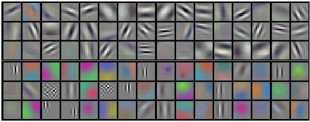
This resemblance might seem weak, but the network was trained on all kinds of natural images (and for a different task), while our dictionary was fit to a specific texture set. Still, you can observe some similar patterns – appearance of edges, fixed color patches, more highly textured regions. It also resembles some other overcomplete frames like Gabor wavelets. I think of it intuitively that as the network also learns some representation of the image (for the given task), those neural network features are also a overcomplete representation, and however they are not sparse, some regularization techniques can partially sparsify them.

Neural networks have mostly replaced sparse methods as they decoupled the slow training from (relatively) fast interference, however I think there is something beautiful and very “interpretable” about the sparse approaches, and when you have already learned a dictionary and don’t need to iterate, for many tasks they can be attractive and faster.

Conclusions

My post aimed to provide some gentle (not comprehensive, but rather a more intuitive and hopefully inspiring) introduction to sparse and dictionary learning methods and why they can be useful and attractive for some image compression and processing tasks. The only novelty is a proposal of using those for compressing PBR textures (again I want to strongly emphasize the idea of exploiting relationships between the channels – if you compress your PBR textures separately, you are throwing out many bits! 🙂 ), but I hope that you might find some other interesting uses. Compressing animations? Compressing volumetric textures and GI? Filtering of partial GI bakes (where one part of level is baked and we use its atoms to clean up the other one)? Compressing meshes? Let me know what you think!