This post is a follow-up to my post on deconvolution/deblurring of the images.

In my previous blog post, I discussed the process of “deconvolution” – undoing a known convolution operation. I have focused on traditional convolution filters – “linear phase, finite impulse response,” the type of convolutional filter you typically think of in graphics or machine learning. Symmetric, every pixel is processed independently, very fast on GPUs.

However, If you have worked with signal processing and learned about more general digital filters, especially in audio – you might have wondered about an omission. I didn’t cover one of the common approaches to filtering signals – recurrent (“infinite impulse response”) filtering. While in graphics those techniques are not very popular, they reappear in literature, often referenced in “generalized sampling” frameworks.

This type of filter has some severe drawbacks (which I will cover) but also genuinely remarkable properties – like exact, finite sample count inversion of convolutional filters. As the name implies, their impulse response is infinite – despite a finite sample count.

Let’s fix my omission and investigate the use of recurrent filters for deconvolution!

In this post, I will:

• Answer why might one want to use an IIR filter.
• Explain how an IIR filter efficiently “inverts” a convolutional filter.
• Elaborate on the challenges of using an IIR filter.
• Propose a gradient descent, optimization, and data-driven method to find a suitable IIR filter.
• Explore the effects of regularizing the optimization process and its data distribution dependence.
• Extend this approach to 2D signals, like images.

Motivation – IIR filters for deconvolution

In this post, I will primarily consider 1D signals – for simplicity and ease of implementation. In the case of 2D separable filters, one can apply analysis in 1D and simply apply it along two axes.  I will mention a solution that can deal with slightly more complicated 2D convolutional kernels in the final part of the post.

For now, let’s consider one of the simplest possible convolution filters – a two-sample box blur of a 1D signal, convolution with a kernel [0.5, 0.5].

In my previous post, we looked at a matrix form of convolution and frequency response. This time, I will write it in an equation form:

When written like this, to deconvolve a signal – find the value of , we do a simple algebraic manipulation:

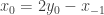
This is already our final solution and a formula for a recurrent filter!

A recurrent filter (Infinite Impulse Response) is a filter in which each sequence value depends on the recurrent filter’s current and past inputs and outputs.

Here is a simplified diagram that demonstrates the difference:

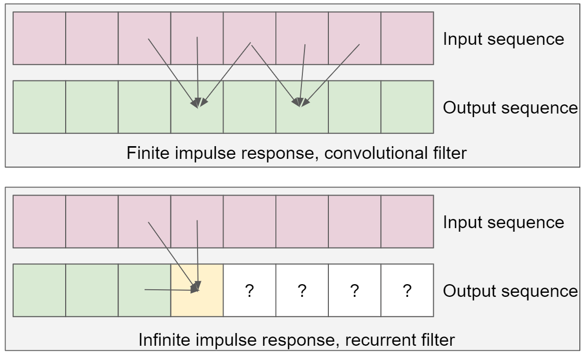
In the above diagram, we observe that in an IIR filter to compute a “yellow” output element, we need the value of the previous output elements in the sequence. This contrasts with a finite impulse response filter – where the output depends only on the inputs, has no output dependence, and we can efficiently process them in parallel.

Implementing an IIR filter and some basic properties

If we were to write such a filter in Python, running it on an input list would be simple for loop:

def recurrent_inverse(seq):
    prev_val = seq[0]
    output = []
    for val in seq:
        output.append(2 * val - prev_val)
        prev_val = output[-1]
    return output

We need to initialize the first previous value to “something,” which depends on the used boundary conditions – often, initializing with the first value of the sequence is a reasonable default.

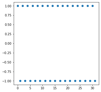
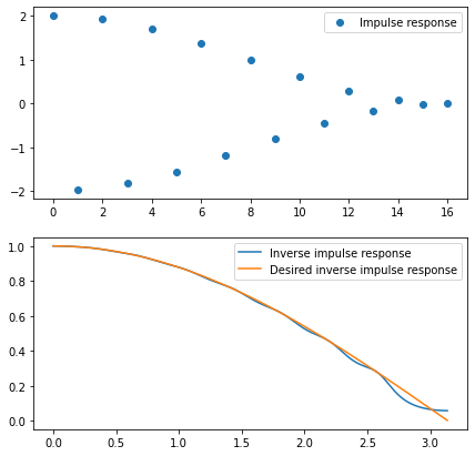
The recurrent filter has some interesting properties. For example, if we plot its impulse response, we get an infinite, oscillating one (hence the name “infinite impulse response”):

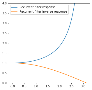
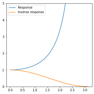
This filter’s frequency response and its inverse are a perfect inversion of the [0.5, 0.5] filter:

The infinite response has a consequence of blowing up the Nyquist frequency to infinity – which we expected, as we are inverting a filter with zero response. If you process a signal consisting purely of Nyquist like:

The result is growing towards oscillating infinity:

This is the first potential problem of IIR filters – instability resulting from the signal processing  concept of “poles.” Suppose the processed signal contains unexpected data (like frequencies not supposed to be present from the blurring). In that case, the result can be an infinite singularity and very quickly overflow numerically!

While I have solved this equation “by hand,” it’s worth noting that there is a neat linear algebra solution and connection. If we look at the convolution matrix, it’s… lower triangular matrix, and we can compute the solution with Gaussian elimination. This will come in handy in a later section.

Signal processing solutions

If you are interested in finding analytically inverse filters to any “arbitrary” system comprised of FIR and IIR filtering components, I recommend grabbing some dense signal processing literature. 🙂 The keywords to look for are Z-transform and “inverse Z-transform.”
The idea is simple: we can write a system’s response using a Z-transform. Then, some semi-analytical solutions (often involving circular integrals) compute a system with the exact inverse response. Those methods are not very easy and require quite a lot of theoretical background – and to be honest, I don’t expect most graphics engineers to find them very useful. Nevertheless, it’s a fascinating field that helped me solve many problems throughout my career.

The beauty of IIR filters

IIR filters (sometimes called in literature “digital filters,” which is somewhat confusing terminology for me) have the beautiful property of being exceptionally computationally sparse and efficient.

This simple box filter [0.5, 0.5] is complicated to deconvolve using FIR filters – even if we regularize its response to avoid “exploding” to infinity and an infinitely large filter footprint.

Here is an example of inverse, regularized / windowed FIR filter impulse response as well as its frequency response:

I have used (my favorite) Hann window. Even with 17 taps of a filter, the resulting frequency response oscillates and doesn’t fully invert the original filter.

Note: truncating and windowing IIR filter responses is another practical way of finding desired deconvolving FIR filters analytically. I didn’t cover it in my original post (as it requires multiple steps: finding an inverse IIR filter and then truncating and windowing its response), but it can yield a great solution.

Comparing those 17 samples to just two samples of an inverse IIR filter – one past value, and one current value – recurrent filter is significantly more efficient.

This is why IIR filters are so popular when we need strong lowpass or highpass filtering with low memory requirements and low computational complexity. For example, almost all temporal anti-aliasing and temporal supersampling use recurrent filters!

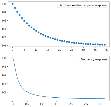
Temporal antialiasing often uses an exponential moving average with a history coefficient of 0.9.

The resulting impulse response and frequency response are:

To get a similar lowpass effect in TAA, like with a recurrent formulation, one would have to use forty history samples, warp all of them according to their motion vectors/optical flow, and weight/reject according to occlusions and data changes. Just holding 40 past framebuffers is infeasible cost memory storage-wise, not to mention the runtime cost!

When a single IIR filter is not enough…

So far, I have used a deceptively simple example of a causal filter – where the current value depends only on the past values (in the [0.5, 0.5] filter, which shifts the image by a half-pixel).

This is the most often used type of filter in signal processing, which comes from the analog, audio, and communication domains. Analog circuitry cannot read a signal from the future! And it’s very similar to the TAA use case, where the latency is crucial, and we produce a new frame immediately without waiting for future ones.

Unfortunately, this is rarely the case for the other filters in graphics like blurs, Laplacians, edge/feature detectors, and many others. We typically want a symmetric, non-causal filter – that doesn’t introduce phase distortions and doesn’t shift the signal/image.

How do we invert a simple, centered [0.25, 0.5, 0.25] binomial filter? The center value “has to” depend both on the “past history” and the “future history”… 

Instead, we can… run a single IIR filter forward and then the same filter backward!

This is suggested in classic signal processing literature and has an interesting algebraic interpretation. When we consider a tridiagonal matrix, we can look at its LU decomposition and proceed to solve it with Gaussian elimination.

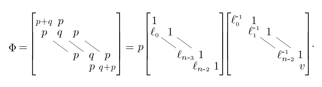
Those methods get complicated and mathematically dense, and I will not cover those. They also don’t generalize to more complex filters in a straightforward manner.

Instead, I propose to use optimization and solve it using data-driven methods.

We will find a pair of backward and forwards recurrent filters just relying on straightforward gradient descent.

The first forward pass will start deconvolving the signal (and slightly shift it in phase), but the real magic will happen after the second one. The second pass not only deconvolves perfectly but also undoes any signal phase shifts:

But first, let me comment on some reasons why it might not be the best idea to use an IIR filter in graphics and some of their disadvantages.

Why are IIR filters not more prevalent in graphics?

IIR filters are one of those algorithms that looks great in terms of theoretical performance – and in many cases, are genuinely performant. But also, it’s one of those algorithms that start to look less attractive when we consider a practical implementation – with implications like limited precision (both in fixed point and in floating point) and the usage of caches and memory bandwidth.

Let’s have a look at some of those. This is not to discourage you from using IIR filters but to caution you about potential pitfalls. This is my research and work philosophy. Think about everything that could go wrong and the challenges along the way. Determine if they could be solved – typically, the answer is yes! – and then confidently proceed to solve them one by one.

Instability

We have already observed how a simple recurrent filter inverting a [0.5, 0.5] convolutional filter can “explode” and go towards infinity on an unexpected sequence of data (frequency content around Nyquist).

In practice, this can happen due to user error, wrong data input, or a very unlucky noise pattern in the sequence. We expect algorithms not completely to break down on an incorrect or unfortunate data sequence – and in the case of IIR filter, even a localized error can have catastrophic consequences!

Imagine the accumulator intermittently becoming floating point infinity or “not a number” value. Then every single future value in the sequence depends on it and will also be corrupted – errors are not localized!

Such an error often occurs in many TAA implementations – where a single untreated NaN pixel can eventually corrupt the whole screen. On “God of War” we were getting QA and artist bug reports that were mysteriously named along the lines of “black fog eats the whole screen.” 🙂

Fixed point implementations generally tend to be more robust in that regard – as long as the code correctly checks for any potential over- or underflows.

Sensitivity to numerical precision

IIR filters rely on the past outputs – thus, any rounding error present in the previous computation might also accumulate, increasing – and eventually potentially “exploding” over time.

Here is an example:

This can be an issue with both fixed and floating point implementations.

This type of error is also highly data-dependent. On one input, the algorithm might perform perfectly, while on another one, the error can become catastrophic.

This is challenging for debugging, testing, and creating “robust” systems.

Limited data parallelism

IIR filters are considered “unfriendly” to a GPU or SIMD CPU implementation. When we process data at the time stamp N, we need to have computed the past values – which is an inherently serial process.

There are efficient GPU or SIMD implementations of the recurrent filters. Those typically rely on either vectorizing along a different axis (in an image, computing the IIR along the x-axis still allows for parallelism on the y-axis), splitting the problem into blocks, and performing most computations in the local memory.

This is significantly more difficult – especially on the GPU – than an FIR filter which can perform close to the performance limits – often even naively computed!

Multiple, transposed passes over data

Finally, the method for bidirectional IIR filters we are going to cover in the next section requires passing over the data in two passes – forward and backward. For separable filtering in 2D, this becomes four passes on both axes.

Even if every pass has minimal amounts of computations, this results in high memory bandwidth cost. By comparison, even large FIR filters – like 21×21 or even more, can go through the data in only a single pass. This matters especially on GPU when using an efficient compute shader or CUDA implementation, which can be extremely fast. This is one of the reasons why the machine learning world switched from recurrent neural networks to using attention layers and transformers for modeling temporal sequences like language or even video.

In image processing, one paper presented an interesting and smart alternative to bilateral filters for tasks like detail extraction or denoising – using recurrent filters for approximating geodesic filtering. Geodesic filters have different properties from bilateral ones and can be desirable in some tasks. Unfortunately, implementation difficulties, complexity of the technique, and performance made it somewhat prohibitive for its intended use (at least on mobile phones).

Data-driven IIR filter optimization

I present an alternative, much more straightforward way of finding a bi-directional recurrent filter that doesn’t require signal processing expertise.

Note: This section and the rest of the post assume the reader is familiar with “optimization” techniques that formulate an objective and solve it using iterative methods like gradient descent. If you are not familiar with those, I recommend reading my post on optimization first. It also introduces Jax as an optimization framework of my choice.

We formulate an optimization problem:

1. Start with some data sequence. Initially, a purely random “white noise” as it contains all the signal frequencies – later, we will analyze the impact of this choice. We will call this target sequence.
2. Apply the convolutional filter you would like to invert to the target sequence. We will call the resulting data input sequence.
3. Write a differentiable implementation of a recurrent filter and a function that runs it on the input data in both directions (forward and backward).
4. Create a differentiable loss function – for example, L2 – between the applied filter on the input sequence and the target sequence. The used loss function will strongly affect the results.
5. Initialize IIR parameters to an “identity” filter.
6. Run multiple iterations of gradient descent on the loss function with regard to the filter parameters. I used simple, straightforward gradient descent, but a higher order method and a dedicated optimizer can perform better.
7. After the optimization converges, we have our bidirectional recurrent filter!

Let’s go through those step by step – but if the concept doesn’t seem familiar, I recommend checking my past blog post on using offline optimization in graphics.

Similar to my past posts, I will use Python and Jax as my differentiable programming framework of choice.

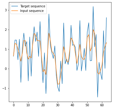
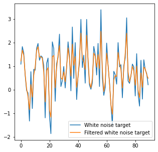
Target and input sequences

This is the most straightforward step. Here is the target sequence (random, Gaussian noise), and an input sequence, convolved with a [1/4, 1/2, 1/4] “binomial” filter, for example:

Differentiable IIR filter and loss function

This part is not obvious – how to do it efficiently and generalize to any number of input and recurrent coefficients. I came up with this implementation:

def unrolled_iir_filter(x: jnp.ndarray, a: jnp.ndarray, b: jnp.ndarray) -> jnp.ndarray:
    if len(b) == 0:
        b = jnp.array([0.0])
    padded_x = jnp.pad(x, (len(a) - 1, 0), mode="edge")
    output = jnp.repeat(padded_x[0], len(b))
    for i in range(len(padded_x) - len(a) + 1):
        aa = jnp.dot(padded_x[i : i + len(a)], a)
        bb = jnp.dot(output[-len(b) :], b)
        output = jnp.append(output, aa + bb)
    return output[-len(x) :]

This is not going to be super fast, but if we need it, Jax allows us to both jit and vectorize it over many inputs.

Application and the loss function are very straightforward, though:

@jax.jit
def apply(x, params):
    first_dir = unrolled_iir_filter(x[::-1], params[0], params[1])
    return unrolled_iir_filter(first_dir[::-1], params[0], params[1])
 
@jax.jit
def loss(params):
    padding = 5
    return jnp.mean(jnp.square(apply(test_signal, params) - target_signal)[padding:-padding])

The only thing worth mentioning here is that I compute the loss ignoring the boundaries of the result as the boundary conditions applied there can distort the results.

Optimize!

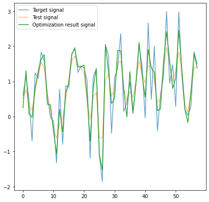
Having everything set up, we run our gradient descent loop. It converges very quickly; I run it for 1000 iterations, taking a few seconds on my laptop. This is how the optimization progresses:

And here is the result, almost perfect!

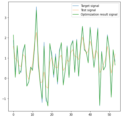
This closeness is remarkable because we cannot recover “some” frequencies (the ones close to Nyquist that get completely zeroed out).

The recurrent filter values I got are 1.77 for the current sample and -0.75 for the past output sample. It’s worth noting that there is an error from the optimization process – those don’t sum to 1.0, but we can correct it easily (normalize the sum). Running the optimization procedure on a larger input would prevent the issue.

When we compute and plot an impulse response of this filter, we get:

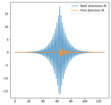
I have plotted two IRs: one after passing through the IIR in the forward direction and then after the backward direction pass.

We observe how the second pass simultaneously symmetrizes the filter and makes the response significantly “stronger,” with much larger oscillations. We can explain the effect of symmetrizing and undoing the phase shifts intuitively – the filter applies the same shifts in the opposite direction – which cancels them out.

Do you have an intuition about the frequency response of the two-pass filter? The frequency response of two passes is the response squared of a single pass:

This comes from the duality of convolution / linear filtering in the spatial domain and multiplication in the frequency domain. 

Here is again the demo of this filtering process happening on an actual signal, first the forwarded pass and then the backward pass:

With two passes, each taking just two samples, we got a recurrent filter equivalent to ~128 samples FIR filter and a squared response of a single recurrent filter!

Plotting the also the inverse response of the combined filter, we get close to the perfect inversion of the [0.25, 0.5, 0.25] filter:

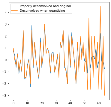
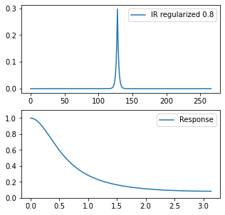
Regularizing against noise

The above response is extreme; it doesn’t go to an infinite boost of the Nyquist frequencies, but in this example, the amplification is ~300. Under the tiniest amount of imprecision, quantization, or noise, it will produce extremely noisy results full of visual artifacts.

Luckily, in this data-driven paradigm regularizing against the noise is as simple as adding some noise before starting the filter coefficient optimization.

test_signal += np.random.normal(size=test_signal.shape) * reg_noise_mag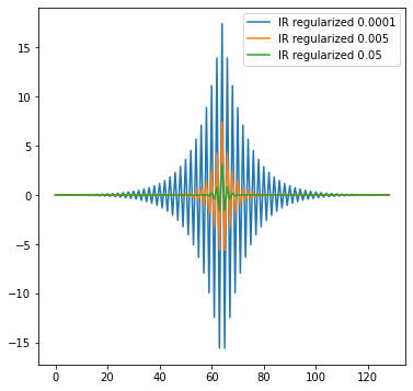

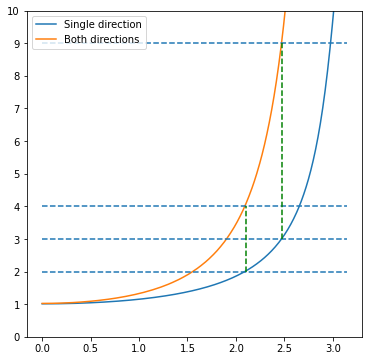
This also caps the maximum frequency response at ~9x boost:

We observe that this regularization smoothens the deconvolution results as well:

What would happen when the noise becomes of a similar magnitude to the original signal?

The data-driven approach automatically learns to get a lowpass, smoothing/denoising filter instead of a deconvolution filter! This can be both a blessing and a curse. Data-adaptive behavior is desirable for practical systems (when the theoretical assumptions and models can be simply wrong). Still, it can lead to surprising behaviors, like wondering, “I asked for a deconvolution filter, not a lowpass filter, this makes no sense.”

Why is the resulting filter lowpass, though, if the noise was 100% white and should contain “all” frequencies? This comes from the per-frequency signal-to-noise ratio. After adding noise to a blurred signal, SNR in those highest frequencies is very close to zero; an optimal filter will remove it. In the lower frequencies (not affected by blur), the amount of noise in proportion to the signal is lower. Thus we need less denoising of those lower frequencies. In my previous post, I described Wiener deconvolution which is an analytical solution that explicitly uses the per-frequency signal-to-noise ratio.

Signal- and data-dependent optimal deconvolution

This naturally brings us to another advantage of data-driven filter generation and optimization. We can use “any” data, not just white noise; more importantly – data that resembles the target use case.

Real data distribution doesn’t look like white noise. For instance, natural images contain significantly more of the lowest frequencies (which is why image downsampling removes detail but can be extreme and we can still tell the image contents).

Similarly, audio signals like speech have a characteristic dominating frequency range of around 1kHz, and our auditory system is optimized for it.

A linear deconvolution filter that is L2-optimal for “natural” images might be very different from the one operating on the white noise! Let’s test this insight.

We will test the original white noise signal with a very subtly filtered version of it (reduced “high shelf” to remove some of the highest frequencies):

After optimizing test signals (both target signals filtered with [0.25, 0.5, 0.25]), we get radically different results and filters:

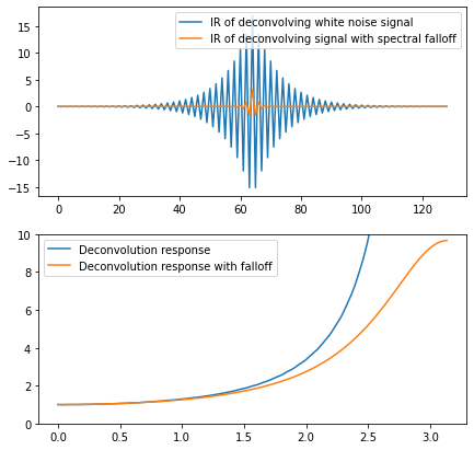
The difference is huge! Even more significant than the one from simply the noise regularization – which might be surprising considering how visually similar both training examples are.

The filter learned on non-white noise is milder and will not create severe artifacts from mild noise or quantization. Its significantly smaller spatial support won’t lead to as noticeable ringing – and won’t “explode” when applied to signals with too much high frequency content.

On the other hand, our perception is very non-linear. Despite images containing not many high frequencies, we are very sensitive to the presence of edges – and an L2 optimized filter ignores this. This is why it is important to model both the data distribution and the loss function correctly representing the task we are solving. 

This lesson keeps reappearing in anything data-driven, optimization, and machine learning. Your learned functions, parameters, and networks are only as good as the training data and the loss function match of the real-world target data and the task being solved. Any mismatch will create unexpected results and artifacts or lead to solutions that “don’t work” outside of the publication realms.

Moving to 2D

So far, my post has focused on 1D signals for ease of demonstration and implementation.

How can one use IIR on 2D images?

Suppose you have a separable filter (like Gaussian). In that case, the solution is simple – running the filter four times – back and forth on the horizontal axis and then on the vertical axis (this generalizes to 3D or 4D data).

Here is a visual demonstration of this process:

Efficiently implementing this on a GPU is not a trivial task – but definitely possible.

Non-separable filters are not easy to tackle – but one can fit a series of multi-pass, different IIR filters. I posted about approximating non-separable shapes with a series of separable filters; here, the procedure would be analogous and automatically learned.

Alternatively, it’s also possible to have a recursion defined in terms of the previous rows and columns. I encourage you to experiment with it – in a data-driven workflow, one doesn’t need decades of background in signal processing or applied mathematics to get reasonably working solutions.

Summary

IIR filters can be challenging to work with. They are sensitive, easily become unstable, are hard to optimize and implement well, require multiple passes over data, and don’t trivially generalize to non-separable filters and 2D.

Despite that, recurrent filtering can have excellent compactness and efficiency – especially for inverting convolutional filters and blurs. They are the bread-and-butter of any traditional and modern audio and signal processing. Without them, graphics’ temporal supersampling and antialiasing techniques wouldn’t be as effective.

In this post, I have proposed a data-driven, learned approach that removes some of their challenges. When learning an IIR filter, we don’t need to worry about complicated algebra and theory, noise, or signal characteristics – and the code is almost trivial. We obtain an optimal filter in a few thousand fast gradient descent iterations. Mean squared error (or any other metric, including very exotic ones, as long as they are differentiable) can define optimality. 

The next step is making those learned filters non-linear, and there are numerous other fascinating uses of data-driven learning and optimization of “traditional” techniques. But those will have to wait for some future posts!