Last year I worked for a bit on a fun research project that ended up published as an arXiv “pre-print” / technical report and here comes a few paragraph “normal language” description of this work.

Neural Networks are taking over image processing. If you only read conference papers and watch marketing materials, it’s easy to think there is no more “traditional” image processing.

This is not true – classical image processing algorithms are still there and running most of your bread and butter image processing tasks. Whether because they get implemented in mobile hardware and each hardware cycle is a few years, or simply due to inherent wastefulness of neural networks and memory or performance constraints (it’s easy for even simple neural networks to take seconds… or minutes to process 12MP images). Even Adobe uses “neural” denoising and super-resolution in their flagship products only in slow, experimental mode.

Misconception often comes from a “telephone game” where engineering teams use neural networks and ML for tasks running at lower resolution like object classification, segmentation, and detection, marketing claims that technology is powered by “AI” (God, I hate this term. Detecting faces or motion is not “artificial intelligence”), and then influencers and media extrapolate it to everything.

Anyway, quality of those traditional algorithms is widely varying and depends a lot on the costly manual tuning process.

So the idea goes – why not use extremely tiny, shallow networks to produce local, per-pixel (though in half or quarter resolution) parameters and see if they improve the results of such a traditional algorithm? And by tiny I mean running at lower resolution, and having less than 20k parameters and so small that it can be trained in just 10 minutes!

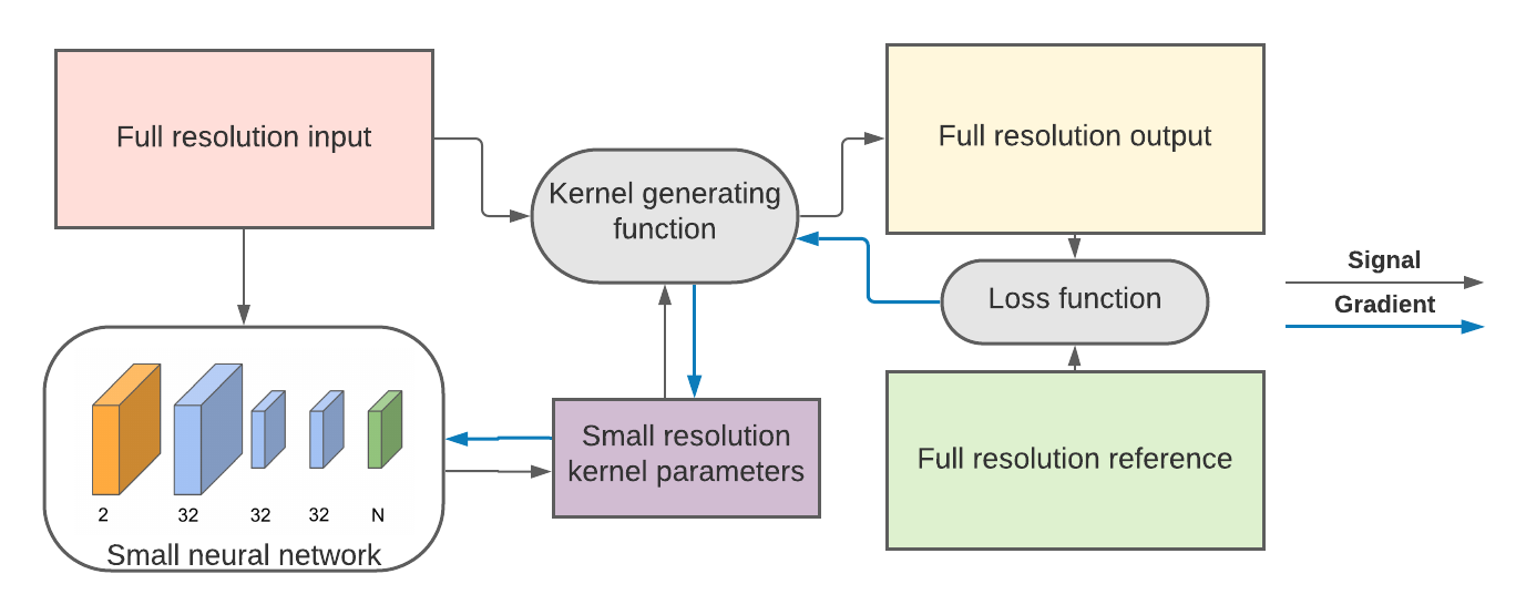
The answer is that it definitely works and it significantly improves results of classic bilateral or non-local means denoising filter. 

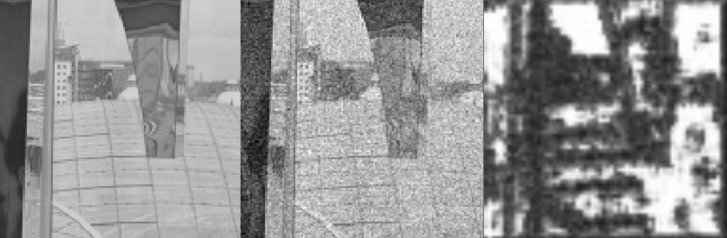
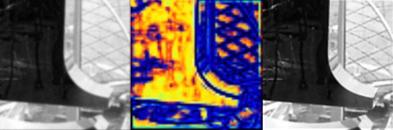
This has a nice advantage of producing interpretable results, which is a huge deal when it comes to safety and accountability of algorithms – important in scientific imaging, medicine, evidence processing, possibly autonomous vehicles. Here is an example of a denoised image and a produced parameter map – white regions mean more denoising, dark regions less denoising:

This is great! But then we went a bit further and investigated the use of different simple “kernels” and functions to generate parameters to achieve tasks of denoising, deconvolution, and upsampling (often wrongly called single frame super-resolution).

First example of a different kernel is using simple Gaussian blur kernel (isotropic and anisotropic) to denoise an image:

It also works very well and produces softer, but arguably more pleasant results than a bilateral filter. Worth noting that this type of kernel is exactly what we used in our Siggraph 2019 work on multi-frame super-resolution, but I spent weeks tuning it by hand… And here an automatic optimization procedure found some very good, locally adaptive parameters in just 10 minutes of training.

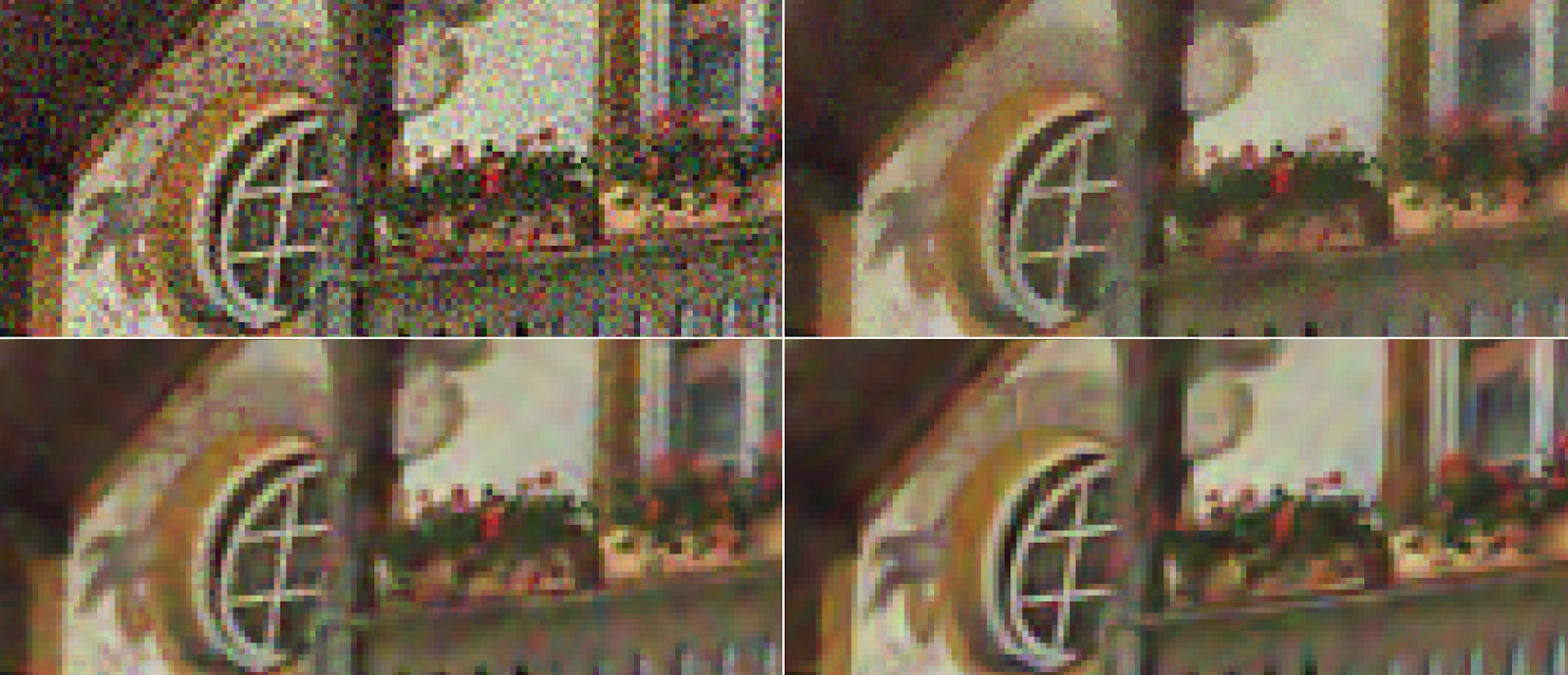
Second application uses polynomial reblurring kernels (work of my colleagues, check it out) to combine deconvolution with denoising (very hard problem). In their work, they used some parameters producing perceptually pleasant and robust results, but again – tuning it by hand. By comparison the approach proposed approach here not only doesn’t require manual tuning, optimizes PSNR, but also denoises the image at the same time!

And it again works very well qualitatively:

And it produces very reasonable, interpretable results and maps – I would be confident when using such an algorithm in the context of scientific images that it cannot “hallucinate” any non-existent features:

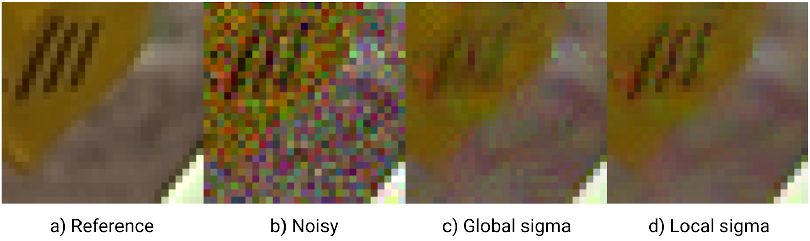
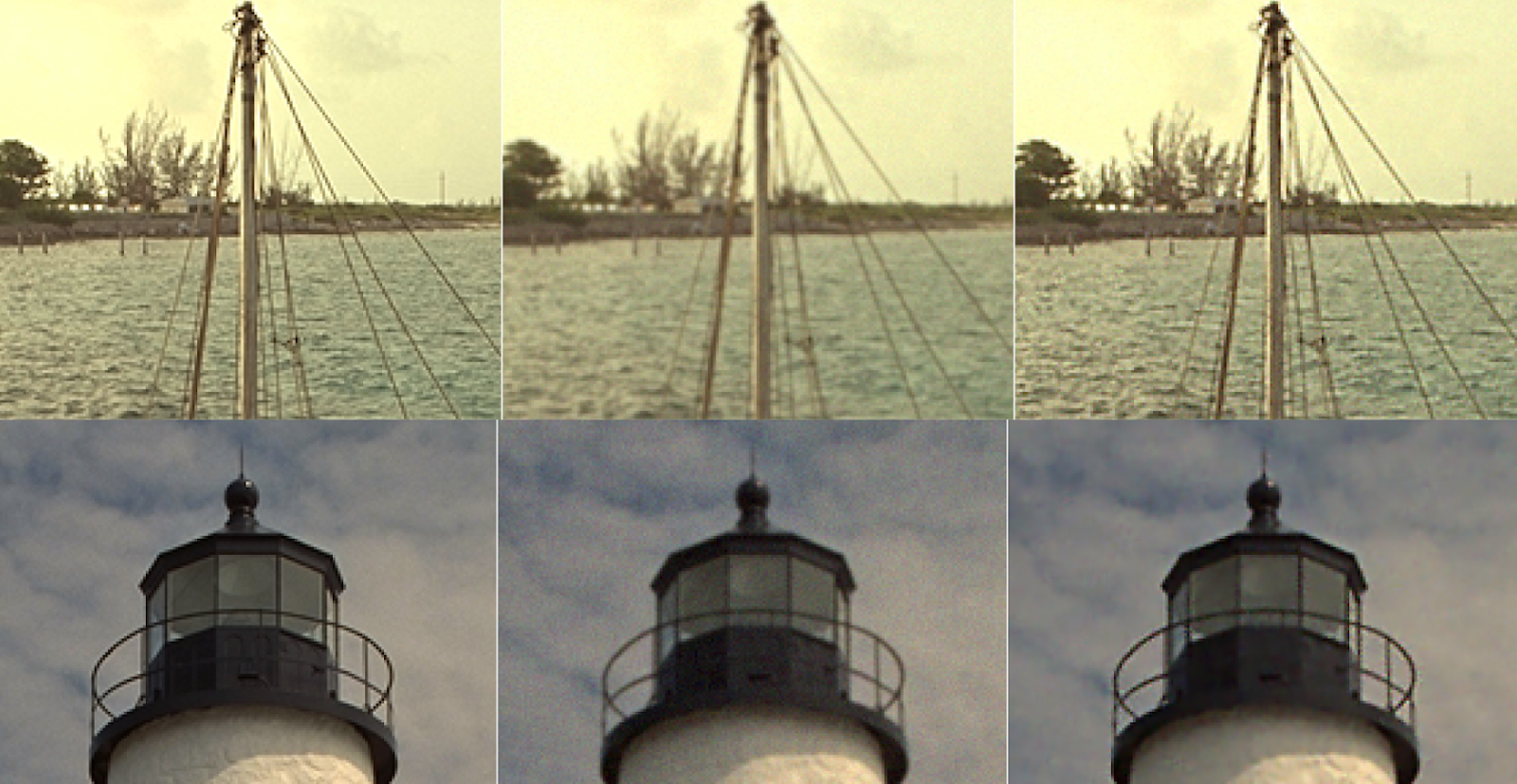
Final application is single frame (noisy) image upsampling (wrongly called often super-resolution). Here I used again anisotropic Gaussian blur kernel, predicted at smaller resolution and simply bilinearly resampling. Such a simple non-linear kernel produces way better results than Lanczos!

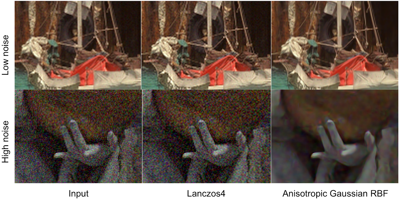
I simply love the visual look of the results here – and note that the same and simple network produced parameters for both results on the right and there was no retraining for different noise levels!

The tech report has numerical evaluations of the first application; some theoretical work on how to combine those different kernels and applications in a single mathematical framework; and finally some limitations, potential applications, and conclusions – so if you’re curious, be sure to check it out on arXiv!