In this post I’ll describe a small hike into the landscape of using linear algebra methods for analyzing seemingly non-algebraic problems, like light transport.

This is very common in some domains of computer science / electrical engineering (seeing everything as vectors / matrices / tensors), while in some others – like computer graphics – more occasional.

Light transport matrices used to be pretty common in computer graphics (for example in radiosity or more broadly, precomputed radiance transfer methods), so if some things in my post seem like rediscovering radiosity methods – they are; and I’ll try to mark the connections.

The first half of the post is very introductory and re-explaining some of the common light transport matrix concepts – while the second half will cover some more interesting and advanced, open ideas / problems around singular value decomposition and spectral analysis of those light transport matrices.

I’ll mention two ideas I had that seemed novel and potentially useful – and spoiler alert – one was not novel (I found prior work that describes exactly the same idea), and the other one is interesting and novel, but probably not very practical.

(While in academia there is no reward for being second to do something, in real life there is a lot of value in the discovery journey you made and idea seeds planted in your head. 🙂 )

And… it’s an excuse to produce some cool, educational figures and visualizations, plus connect some seemingly unconnected domains, so let’s go.

What is light transport and light transport matrix?

Light transport is in very broad, handwavy terms the physical process of light traveling from destination A to destination B and potentially interacting with the environment along the way. Light transport is affected by the presence of occlusions, participating media, angles at which surfaces are to each other, materials that emit or absorb certain amounts of light.

One can say that the goal of rendering is to compute the light transport from the scene to the camera – which is as broad as it gets, this is like almost all computer graphics!

We will simplify and heavily constrain this to a toy problem in a second.

Light transport matrices

Before describing the simplifications we will make, let’s have a look at how light transport could be represented in an extremely simple scene that consists of three, infinitesimal (infinitely small) points A, B, C. Infinitesimal / differential elements are very common in light transport – we assume they have a surface, we compute light transport on this surface, but this surface goes asymptotically towards 0, so we can ignore integrating over this surface.

If we “somehow” compute how much light gets emitted from the point A to point B and C, from point B to A and C, and C to A and B, we can represent it in a 3×3 matrix:

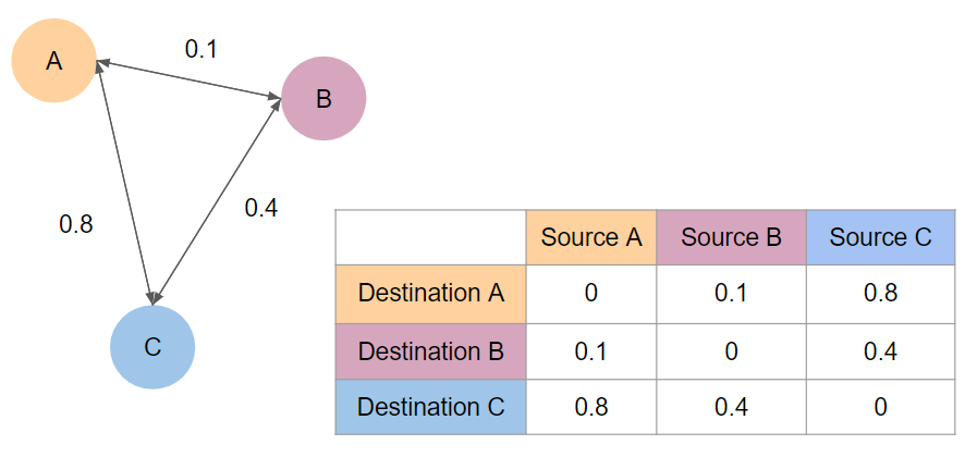
A few things to note here: in this case, we look only at a single bounce of light – therefore values on the diagonal are zero – shining some light on point A doesn’t transmit any light to itself through any other paths.

In this case, the presented matrix is symmetric – we assume the same amount of light gets transmitted from A to B and from B to A.

This doesn’t need to be the case – there can definitely be some non symmetric matrices present, though many of their “components” and elements that contribute to their values are symmetric.

If point A has no direct path to point B, point B also won’t have a path to point A.

Thus a visibility or shadowing term of a direct light transport matrix would be similar.

The same goes for so-called form factor (or view factor).

I will not go too much into the form factor matrix, but it is interesting that assuming full, perfect discretization and coverage of the scene it is not only strictly positive, symmetrical, but also double stochastic matrix – all rows and columns sum to 1.0.

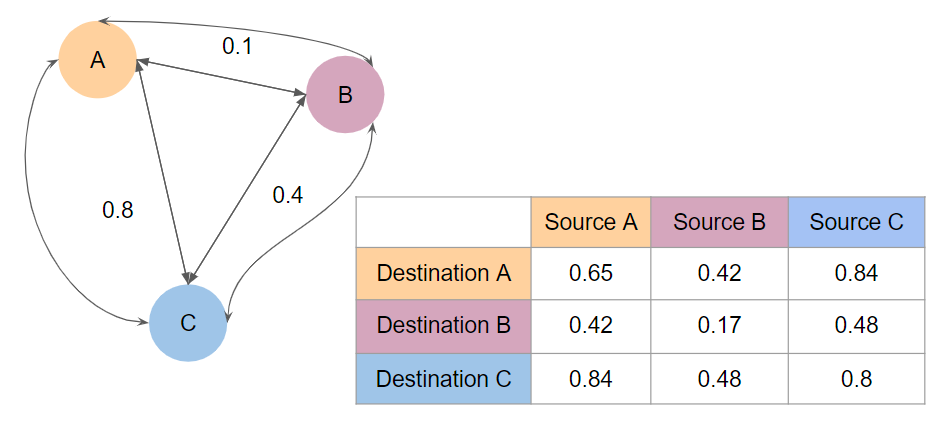
We have a light transport matrix… Why is it useful? It allows us to express interesting physical interactions by simple mathematical operations! One example (more on that later) is that by computing M + M @ M – a matrix addition and multiplication – one can express computation of two bounces of light in the scene.

We can also compute the lighting in the scene when we treat point A as emitting some light.

Assuming that we put there 1.0, we end with a simple matrix – vector multiplication like:

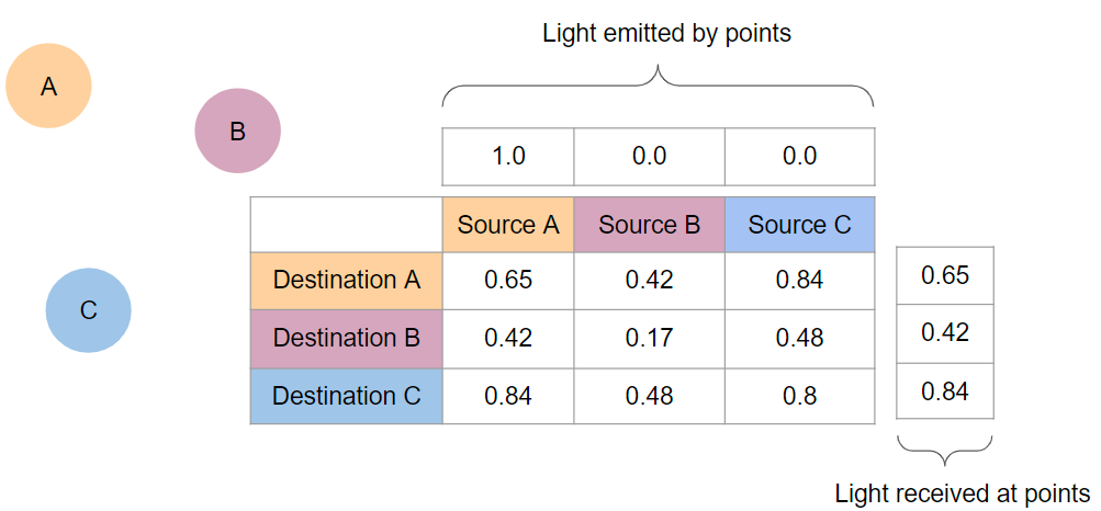
So with a single algebraic operation, we computed light received at all points of the scene after two bounces of GI lighting.

Assumptions and simplifications

Let’s make the problem easy to explain and play with by doing some very heavy simplifications and assumptions I’ll be using throughout the post:

• I will assume that we are looking only at a single wavelength of light – no colors involved,
• I will look at a 2D slice of the problem to conveniently visualize it.
• I will assume we are looking only at perfectly diffuse surfaces (similar to radiosity),
• I will assume everywhere perfectly infinitesimal single points (no area),
• I will be very loose with things like normalization or even physicality of the process,
• I will assume that the used occluder is a perfect black hole – absorbs all light and doesn’t emit anything. 🙂 
• When displaying results of “lighting”, I will perform gamma correction, when visualizing matrices not. 

Computing a full matrix

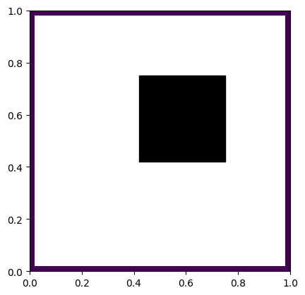
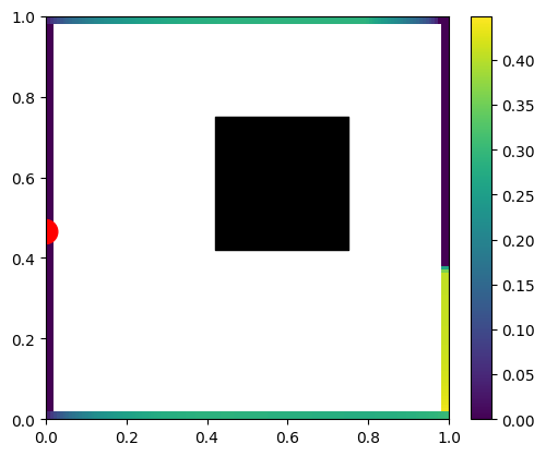
Let’s start with a simple scene – a closed box that has diffuse reflective surfaces, and in the middle of the box we have a “black hole” with a rectangular event horizon that captures all the light on its ways, something like:

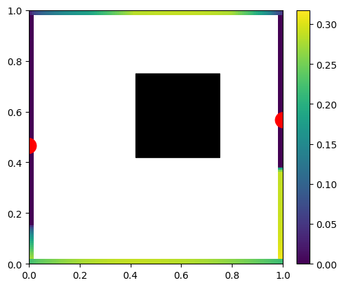
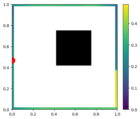
Now imagine that we diffusely emit the light from just a single, infinitesimal point of the scene.

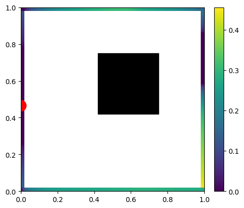
We’d expect to get something like this:

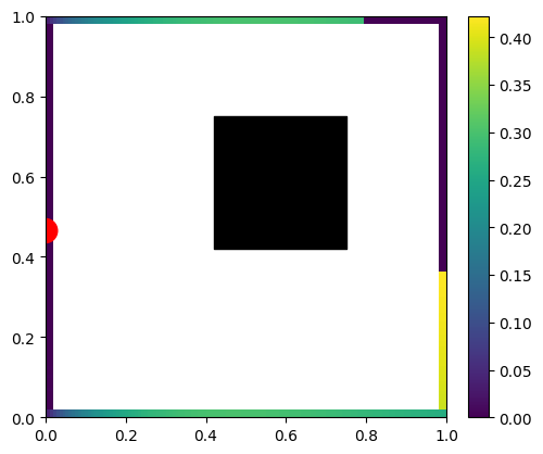
A few things to notice – the wall with light on it (red dot) doesn’t get any light to any point on the wall due to the form factor (multiplication of cosine angles between two points normals and the path direction) being 0.0. This is the “infamous cosine component of Lambertian BRDF” – infamous as the Lambertian BRDF itself is constant; the cosine term comes from surface differentials and is a part of any rendering equation evaluation.

Other surfaces follow a smooth distribution, but we can also see directly some hard shadows behind our black hole.

How do we compute the light transport though? In this case, I have discretized the space. Each wall of the box gets 128 samples along the way:

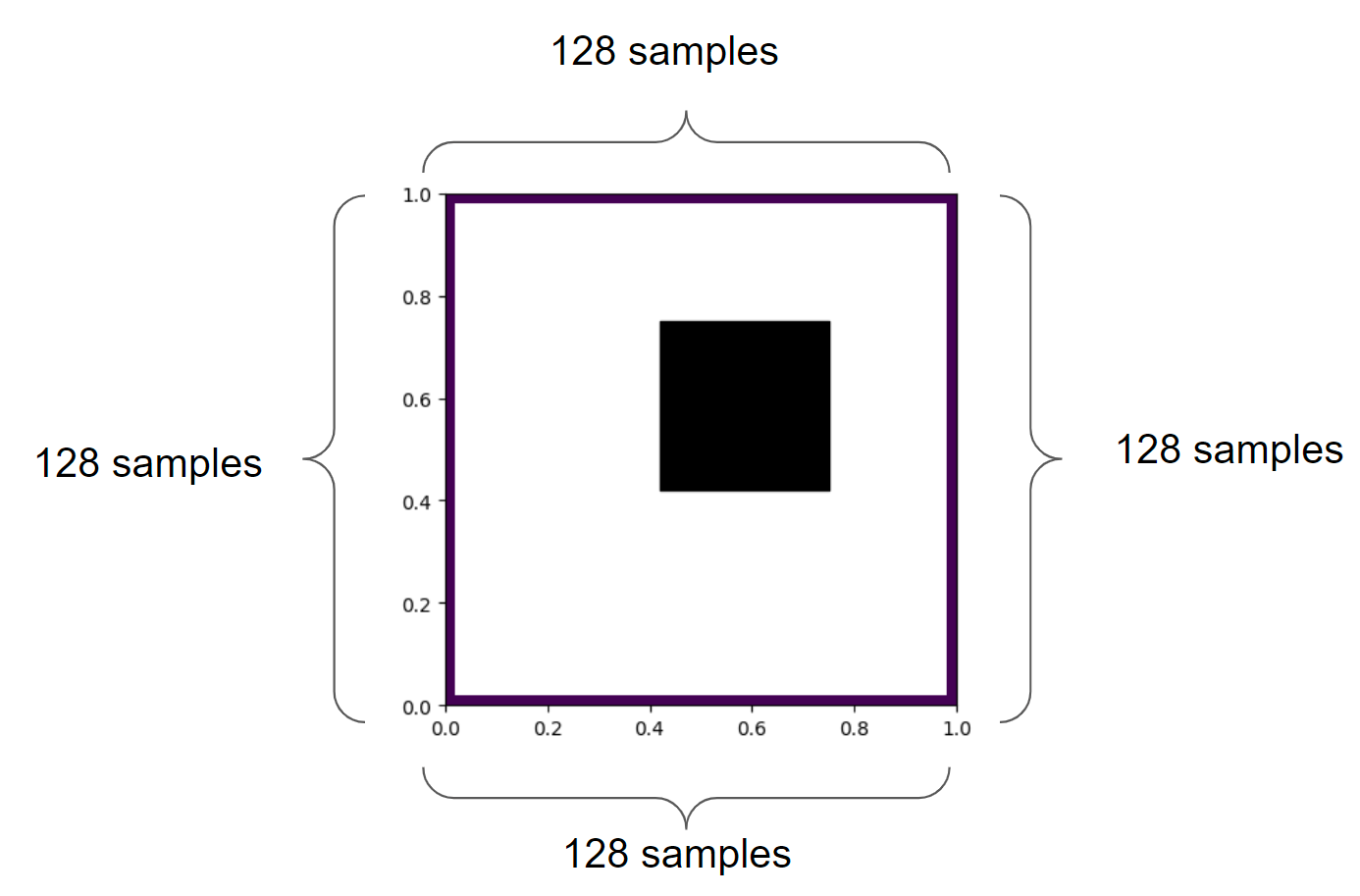
We have 4 x 128 == 512 points in total.

The light transport matrix – which describes the amount of light going from one point to the other – will have 512 x 512 entries.

This already pretty large matrix will be a Hadamard (elementwise) product of three matrices:

• Form factors (depending on the surface point view angles),
• Shadowing (visibility between two patches),
• Albedo.

I will use a constant albedo of 0.8 for all of the patches.

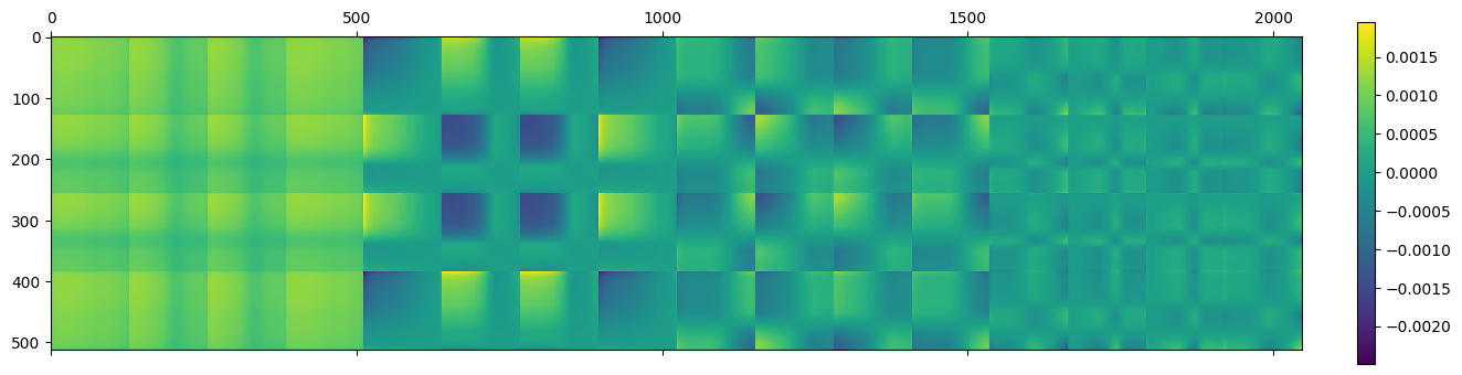
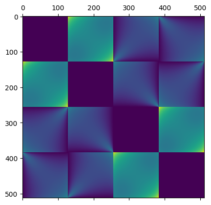
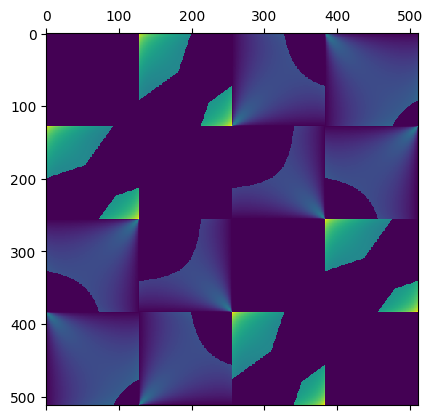
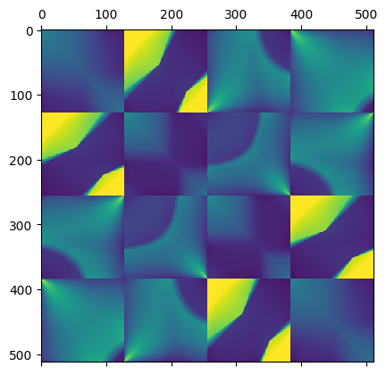
The form factor matrix has a very smooth, symmetric and block form:

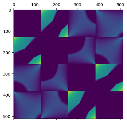
And if we multiply it by shadows (whether a path from point A to point B intersects the “black hole”) we get this:

Notice how the hard shadows simply “cut out” some light interaction between the patches.

We can soften them a little bit (and it will be useful in a bit, improving low rank approximations):

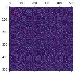
Very important: that the matrix looks so nice only because elements are arranged “logically” – 4 walls after one another, sorted by increasing coordinates.

The elements we compute the transport between can be in any order, so for example the above “nice” matrix is equivalent to this mess (I randomly permuted the elements):

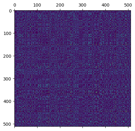
Keep this in mind – while we will be looking only at “nicely” structured transport matrices to help build some intuition, same methods work on “nasty” matrices.

Ok, so we have a relatively large matrix… in practical scenarios it would be gigantic, so big that often it’s prohibitive to compute or store.

We will address this in a second, but first – why did we compute it in the first place?

Using the matrix for light transfer

As mentioned above, having this matrix, computing transfer from all points to all the other points becomes just a single matrix-vector multiplication.

So for example to produce this figure:

I took a vector full of zeros – for all the discrete elements in the scene – and put a single “large” value corresponding to light diffusely emitted from this point.

Computing a full matrix for just a single point would be super wasteful though; we could have computed it directly.

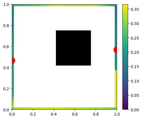
The beauty comes from being able to use the same light transport matrix can handle 2 or 3 light sources – and it is still the same matrix computation and can be reused:

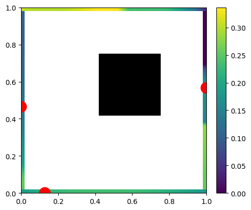
Again, using just 2 or 3 lights is a bit wasteful, but nothing prevents us from computing area lights:

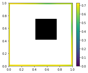
…or if the final lighting values if every single point in the scene was lightly emissive:

Light transport matrices are useful for example for precomputed light transport and computing the light coming into the scene from image-based lighting (like cubemaps).

Algebraic multi-bounce GI

Even better property comes from looking again at a simple question: “what is the meaning of light transport of the light transport?” (matrix multiplication) – it is the same as multiple bounces of light!

Energy from an Nth bounce is simply M * M * M …, repeated N times.

Thus, total energy from N bounces can be written as either:

M + M * M + M * M * M + …

Or alternatively ((M+I)*M+I)*M*…

We are guaranteed that if the rows and columns that are positive and sum to below 1.0 (and they have to be! We cannot have an element contributing more energy to the scene than it receives) and more formally, that singular values are below 1 (more about it in the next section), this is the same as geometric series and will converge.

How do those matrices look like? This is the 1st, 2nd and 3rd bounce of light (I bumped up the scale a bit to make the 3rd bounce more visible):

We can observe that already the 3rd bounce of light doesn’t contribute almost any energy.

Also due to the regular structure of the matrix itself, the structure of the bounces gives us some insight.

For example – while the 1st bounce of light doesn’t shine anything onto patches on the same wall (blocks around the diagonal), the 2nd bounce contributes the most energy – light bouncing back and straight.

Another observation is that every next bounce is more blurry / diffuse. This also has interesting spectral (singular value) interpretation (I promise we’ll get to that soon!).

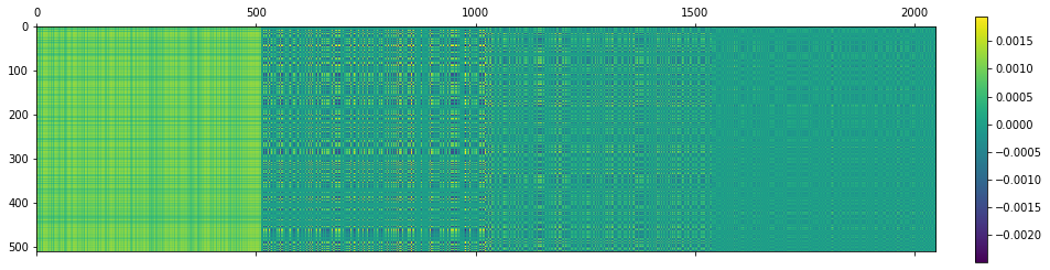
When we sum up the first 5 bounces of light, we’d get a matrix that looks somewhat like:

…And now we can use this newly computed light transport matrix to visualize multi-bounce GI in our toy scene:

Here it is animated to visualize the difference better:

Multiple bounces both add some energy (maximum values increasing), as well as “smoothens” its spatial distribution.

We can do the same with more lights:

Low rank / spectral analysis

After such a long intro, it’s time to get into what was my main motivation to look at those light transport matrices in the first place.

Inspired by spectral mesh methods and generally, eigendecomposition of connectivity and Laplacian matrices, I thought – wouldn’t it be cool to try a low rank approximation of the light transport matrix?

I wrote about low rank approximations twice in different contexts:

• Computing separable approximations of image filters,
• Using correlation present in natural materials to compress whole texture sets.

If you don’t remember much about singular value decomposition, or it is a new topic for you, I highly recommend at least skimming the above.

This random idea seemed very promising. One could store only N first singular values, ignore the high frequency and do some other cool stuff!

There is prior work…

But… as it usually happens when someone outside of the field comes up with an idea – such ideas obviously were explored before.

Two immediate finds are “Low-Rank Radiosity” by E.Fernández and follow-up work with their colleagues “Low-rank Radiosity using Sparse Matrices”. I am sure there is some other work as well (possibly in the radiosity for physics, but those publications are impenetrable for me).

This doesn’t discourage me or invalidate my personal journey to this discovery – the opposite is true.

In general, my advice is to not be discouraged by someone discovering and/or publishing an idea sooner – whatever you learned and built the intuition by doing it yourself is yours. It doesn’t invalidate that you discovered it as well. And maybe you can add some of your own experiences and discoveries to expand it.

Edit: Some of my colleagues mentioned to me another work on low rank light transport, “Eigentransport for Efficient and Accurate All-Frequency Relighting” by Derek Nowrouzezahrai and colleagues and I highly recommend it.

Decomposition of a light transport matrix

What happens if we attempt eigenanalysis (computing eigenvectors and eigenvalues), or alternatively singular value decomposition of the light transport matrix?

(I will use the two interchangeably, as due to matrices in this case being normal, eigendecomposition always exists and can be done through singular value decomposition)

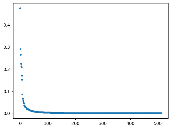
As we expect, we can observe very fast decay of the singular values:

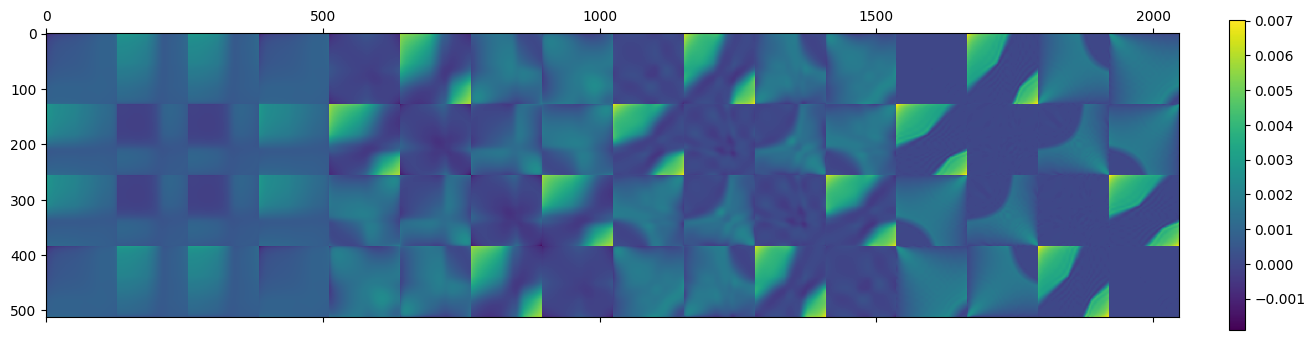
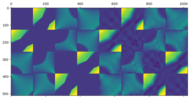
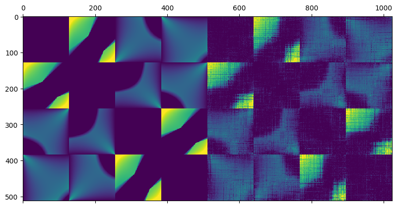
Now, let’s visualize the first few components – I picked 1, 2, 4, 16:

Something fascinating is happening here – notice how we get higher and higher “block” frequency behavior for the matrices corresponding to rank-1 increasing singular values. Additionally, the first component here is almost “flat” and strictly positive, while the next ones include negative oscillations!

Doesn’t this look totally like some kind of Discrete Cosine Transform matrix or generally, Fourier analysis?

This is not a coincidence – both are special cases of applications of spectral theorem.

Discrete Fourier Transform is a diagonalization (computing eigendecomposition) of a circulant matrix (used for circular convolution) and here we compute the diagonalization of a light transport matrix. So called “spectral methods” involve data eigendecomposition, usually of some kinds of Laplacians or connectivity matrices.

Math formalism is not my strongest side – but the simple, intuitive way of looking at it is that generally those components will be orthogonal to each other, sorted by their energy contribution, and represent different signal frequencies present in the data. For most “natural” signals – whether images or mesh Laplacians – with increasing frequency components, singular values very quickly decay to zero.

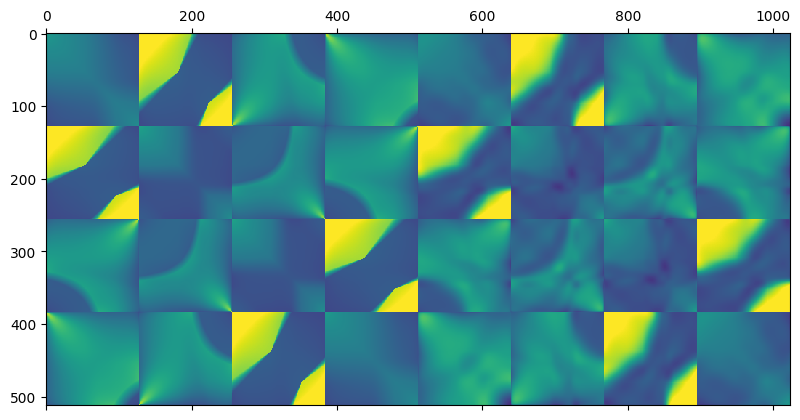
Here are the first 2, 4, 8, 64 components added together:

This is – not coincidentally – very similar to truncating Fourier components.

The shape of the matrix very quickly starts to resemble the original, non compressed matrix.

With 64 components (1/8th squared == 1/64th of the original entries) we get a very good representation, albeit with standard spectral decomposition problems – ringing (see the “ripples” of oscillating values around the harsh transition areas).

When computing the lighting going through the matrix, the results look plausible with as low coefficient count as 8!

I will emphasize here one important point – that “visually pleasant” and interpretable low rank approximation of the matrix is only because we arranged elements “logically” and according to their physical proximity.

This matrix:

…has the same singular values, but the first few components don’t look as “nice”:

(Though arguably one can notice some similar behaviors.)

Both the beauty and difficulty of linear algebra is that those methods work equally well for such “nice” and “bad” matrices, we don’t need to know their contents – though a logical structure and a good visualization definitely helps to build the intuition.

Multi-bounce rank

This was a spectral decomposition of the original, single bounce, light transport matrix.

But things get “easier” if we include multiple bounces. Remember how we observed that multi-bounce causes the matrix (as well as its application results) to be more “smooth”?

We can observe it as well by looking at N bounces singular value distribution:

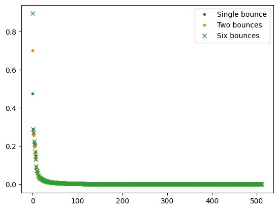
To understand why it is this way, I think it’s useful to think about singular values and matrix multiplication. Generally, matrix multiplication can only lower the matrix rank.

If all singular values are below 1.0, it will also cause them to lower their values after multiplication.

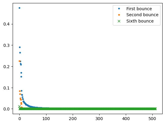
With perfect eigendecomposition, we can go even further and say that they are going to get squared, cubed etc.

It’s worth thinking for a second about why we know that a singular value will always be lower than 1.0? My best “intuitive” explanation is that if the light transport matrix is physically correct, there is no light input vector that will cause more energy to get out of the system than we put into it.

Any singular value that is very low energy will decay to zero very quickly when multiplying the matrix by itself.

This means that a low rank approximation of the multi-bounce light transport matrix is going to be more faithful (as in smaller relative error) to the original one as compared to a single bounce.

It’s even better when looking at the final light transport results:

With only 8 components, the results are obviously not as “sharp” as original, but overall distribution seems to match and be preserved relatively well.

Compressed sensing and matrix completion algorithms?

A second idea that brought me to this topic was reading about compressed sensing and matrix completion algorithms. I will not claim to be any expert here – just have interest in general numerical methods, optimization, and fun algebra.

General idea is that if you have prior knowledge about signal sparsity in some domain (like strong spectral decay!), you could get away with significantly less (random, unstructured) samples, and reconstruct the signal afterwards. Reconstruction is typically very costly, involves optimization, and such methods are mostly a research field for now.

From a different angle, all big tech companies use recommendation systems that have to deal with missing user preference data. If I have only watched and liked one James Bond movie, and one Mission Impossible movie, the algorithm should be able to give me as good a recommendation as if I watched an end-to-end whole James Bond movie collection. In practice, it’s not easy – both to deal with databases of hundreds of millions of users, as well as tens of thousands of movies, some of them very niche. This is obviously a deep field that I lack expertise in – so treat it as a vast (over)simplification.

One of the simpler approaches predating the deep learning revolution was low-rank matrix completion. Core idea is simple – assumes that only a few factors decide that we’re going to watch and like a movie – for example we like spy movies, action cinema, and Daniel Craig. Each user has preferences around some “general” themes, and each movie represents some of those general themes – and it is discovered in a data driven way.

Edit: Fabio Pellacini mentioned to me of prior work with his colleagues, “Matrix Row-Column Sampling for the Many Light Problem” that tackles the same problem through matrix row and column (sub)sampling using low rank assumption. A different (not strictly compressed sensing related method), but very interesting results from a 2007 paper that spawned some follow-up ones!

Edit 2: Another great find comes from Peter-Pike Sloan and it’s a fairly recent work from Wang and Holzschuch “Adaptive Matrix Completion for Fast Visibility Computations with Many Lights Rendering” which is exactly about this topic and idea.

Light transport matrix completion

I toyed around with the idea of how good those algorithms could be for light transport matrix completion?

What if we cast rays and do computations only for for example 20% entries in the matrix?

Note: I have not used the knowledge of form factors, importance sampling, stratified distributions or blue noise etc. which would make it much better. This is as dumb and straightforward application of this idea for demonstration purposes as it gets.

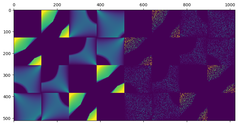
This is the matrix to complete:

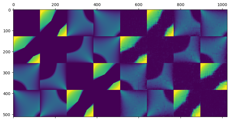
And after optimizing for the matrix completion to find the missing entries through gradient descent (yes, there are some much better/faster methods; for example check out this paper – but this was the easiest to code up and fast enough with such a matrix) to minimize the sum of the absolute singular values (known as nuclear norm) as a proxy for 0-norm, we get something like this:

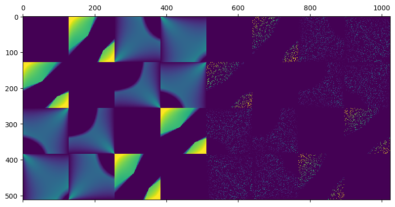
This is actually not too bad! Note that it might seem obvious here how the structure should look like. But in practice, if you get a matrix that looks like this:

Can you figure out its completion if you were to discard 80% of the values? Probably not, but a low rank algorithm can. 🙂 And it would be exactly equivalent to the matrix earlier!

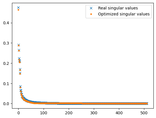
Note how remarkably close are the found singular values to the original ones:

When applied to the scene, it looks “reasonably”:

Things start to fall off the cliff with below 10% of kept values:

…but on the other hand it’s still not too bad!

We didn’t incorporate any rendering domain knowledge, priors or constraints (like knowing that neighboring spatial values should be similar; or that entries with a form factor of 0 have to be 0).

We just rely on some abstract mathematical Hilbert spaces properties that allow for spectral decomposition and the assumption of sparsity and low rank!

This makes the whole field of compressed sensing feel to me like the modern day equivalent of “magic”.

Summary

To conclude, we have looked at light transport matrices, and how they relate to some graphics light transport concepts.

Computing incident lighting becomes matrix-vector multiplication, while getting more bounces is simple matrix multiplication / squaring, and we can sum multiple bounces by summing together those matrices – simple algebraic operations correspond to physical processes.

We looked at the singular value distributions and spectral properties of those matrices, as well as low rank approximations. 

Finally, we played with an idea of light transport matrix completion – knowing nothing about physics or light transport, only relying on those mathematical properties!

Is any of this useful in practice? To be honest, probably not – for sure not by looking at those really huge matrices. But some spectral methods could be definitely applicable and help find “optimal” representations of the light transport process. They are an amazing analysis and intuition building tool.

And as always, I hope the post was inspiring and encouraging your own experiments.