Last week I saw Daniel Holden tweeting about Savitzky-Golay filters and their properties (less smoothing than a Gaussian filter) and I got excited… because I have never heard of them before and it’s an opportunity to learn something. When I checked the wikipedia page and it mentioned it being a least squares polynomial fit, yet yielding closed formula linear coefficients, all my spidey senses and interests were firing!

Convolutional, linear coefficients -> means we can analyze their frequency response and reason about their properties.

I’m writing this post mostly as my personal study of those filters – but I’ll also write up my recommendation / opinion. Important note: I believe my use-case is very different than Daniel’s (who gives examples of smoothed curves), so I will analyze it for a different purpose – working with digital sequences like image pixels or audio samples.

(If you want a spoiler – I personally probably won’t use them for audio or image smoothing or denoising, maybe with windowing, but think they are quite an interesting alternative for derivatives/gradients, a topic I have written before).

Savitzky-Golay filters

The idea of Savitzky-Golay filters is simple – for each sample in the filtered sequence, take its direct neighborhood of N neighbors and fit a polynomial to it. Then just evaluate the polynomial at its center (and the center of the neighborhood), point 0, and continue with the next neighborhood. 

Let’s have a look at it step by step.

Given N points, you can always fit a (N-1) degree polynomial to it.

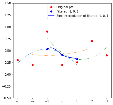
Let’s start with 7 points and a 6th degree polynomial:

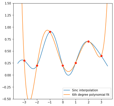
Red dots are the samples, and the blue line is sinc interpolation – or more precisely, Whittaker–Shannon interpolation, standard when analyzing bandlimited sequences.

It might be immediately obvious that the polynomial that goes through those points is… not great. It has very large oscillations. 

This is known as Runge’s phenomenon and equispaced points (our original sampling grid) generally don’t fit polynomials to many functions well, especially with higher polynomial degrees. Fitting high degree polynomials to arbitrary functions on equispaced grids is a bad idea…

Fortunately, Savitzky-Golay filtering doesn’t do this.

Instead, they find a lower order polynomial that fits the original sequence the best in least-squares sense – the sum of squared distances between the polynomials sampled at the original points is minimized.

(If you are a reader of my blog, you might have seen me mention least squares in many different contexts, but probably most importantly when discussing dimensionality reduction and PCA)

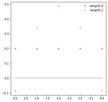
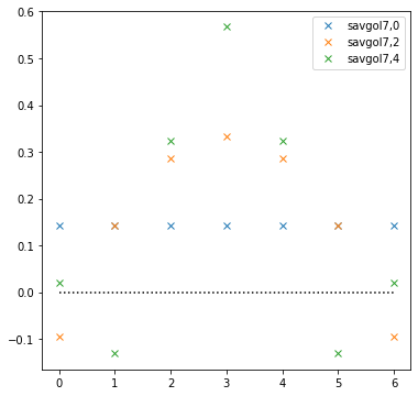
Since this is a linear least squares problem, it can be solved directly with some basic linear algebra and produces following fits:

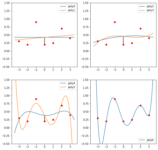
On those plots, I have marked the distance from the original point at zero – after all, this is the neighborhood of this point and the polynomial fit value will be evaluated only at this point.

Looking at these plots there’s an interesting and initially non-obvious observation – degrees in pairs (0,1), (2,3), (3,4) have exactly the same center value (at x position zero). Adding a next odd degree to the polynomial can cause “tilt” and changes the oscillations, but doesn’t impact the symmetric component and the center.

For the Savitzky-Golay filters used for filtering signals (not their derivatives – more on it later), it doesn’t matter if you take the degree 4 or 5 – coefficients are going to be the same.

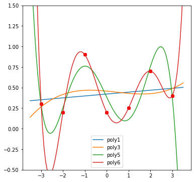
Let’s have a look at all those polynomials on a single plot:

As well as on an animation that increases the degree and interpolates between consequential ones (who doesn’t love animations?):

The main thing I got from this visualization and playing around is how lower orders not only fit the sequence worse, but also have less high frequency oscillations.

As mentioned, Savitzky-Golay filter repeats this on the sequence of “windows”, moving by single point, and by evaluating their centers – obtains the filtered value(s).

Here is a crude demonstration of doing this with 3 neighborhoods of points in the same sequence – marked (-3, 1), (-2, 2), (-1, 3) and fitting parabolas to each.

Savitzky-Golay filters – convolution coefficients

The cool part is that given the closed formula of the linear least squares fit for the polynomial and its evaluation only at the 0 point, you can obtain a convolutional linear filter / impulse response directly. Most signal processing libraries (I used scipy.signal) have such functionality and the wikipedia page has neat derivation.

Plotting the impulse responses for bunch of 7 and 5 point filters:

The degree of 0 – an average of all points – is obviously just a plain box filter.

But the higher degrees start to be a bit more interesting – looking like a mix of lowpass (expected) and bandpass filters (a bit more surprising to me?).

It’s time to do some spectral analysis on those!

Analyzing frequency response – comparison with common filters

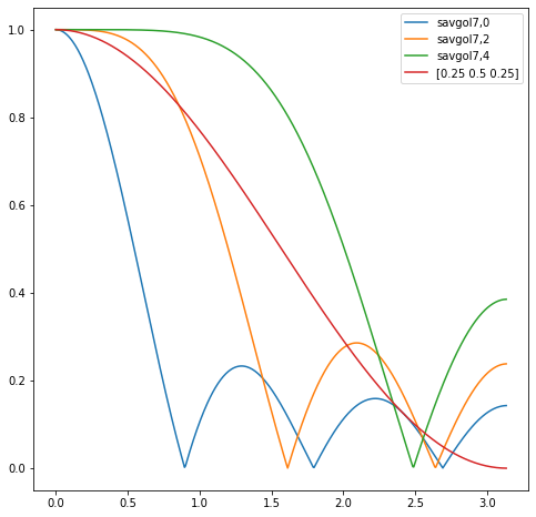
If we plot the frequency response of those filters, it’s visually clear why they have smoothing properties, but not oversmoothing:

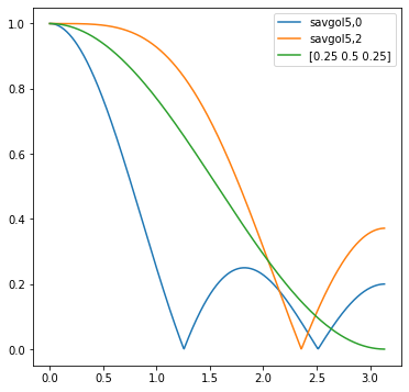
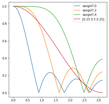
As compared to a box filter (Savgol filters of degree 0) and a binomial/Gaussian-like [0.25, 0.5, 0.25] filter (my go to everyday generic smoother – be sure to check out my last post!), they preserve a perfectly flat frequency response for more frequencies.

What I immediately don’t like about it, is that, similarly to a box filter, it is going to produce an effect similar to comb filtering, preserving some frequencies and filtering out some others – oscillating frequency response; they are not lowpass filters. So for example a Savgol filter of 7 points and degree 4 is going to leave zero frequencies at 2.5 radians per cycle, while leaving out almost 40% at Nyquist! Leaving out frequencies around Nyquist often produces “boxy”, grid-like appearance.

When filtering images, it’s definitely an undesirable property and one of the reasons I almost never use a box filter.

We’ll see in a second why such a response can be problematic on a real signal example.

On the other hand, preserving some more of the lower frequencies untouched could be a good property if you have for example a purely high frequency (blue) noise to filter out – I’ll check this theory in the next section (I won’t spoil the answer, but before you proceed I recommend thinking why it might or might not be the case).

Here’s another comparison – with IIR style smoothing, classic simple exponential moving average (probably the most common smoothing used in gamedev and graphics due to very low memory requirements and great performance – basically output = lerp(new_value, previous_output, smoothing) ) and different smoothing coefficients.

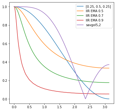
What is interesting here is that the Savitzky-Golay filter is a bit “opposite” of its behavior – keeps much more of the lower frequencies, decays to zero at some points, while IIR never really reaches a zero.

Gaussian-like binomial filter on the other hand is somewhere in between (and has a nice perfect 0 at Nyquist).

Example comparison on 1D signals

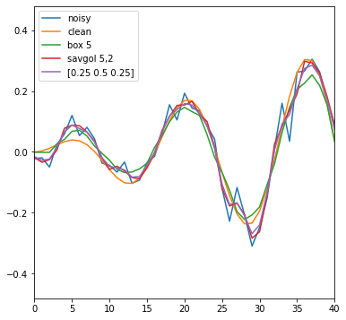
On relatively smooth and smaller filter spatial support signals, there’s not much difference between higher degree savgol and “Gaussian” (while the box filter is pretty bad!):

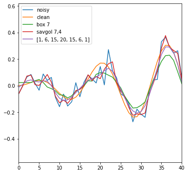
While on more noisy signals and higher spatial support, they definitely show less rounding of the corners than a binomial filter:

On any kind of discontinuity it also preserves the sharp edge, but…

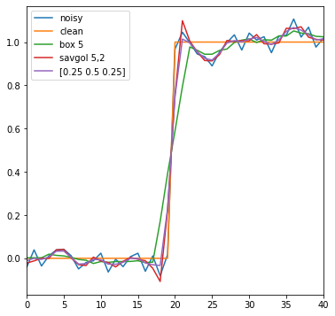
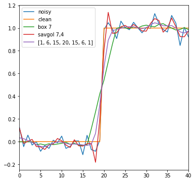
Looks like the Savitzky-Golay filter causes some overshoots. Yes, it doesn’t smoothen the edge, but to me overshooting over the value of the noise is a very undesirable behavior; at least for images where we deal with all kinds of discontinuities and edges all the time…

Example comparison on images

…So let’s compare it on some example image itself.

Note that I have used it in separable manner (convolution kernel is an outer product of 1D kernels; or alternatively applying 1D in horizontal, and then vertical direction), not doing the regression on a 2D grid.

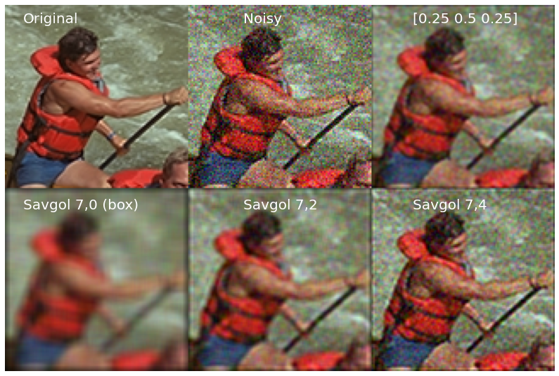
…On the first glance, I quite “perceptually” like the results for the sharpest Savitzky-Golay filter…

…on the other hand, it makes the existing oversharpening of the image from Kodak dataset “wider”. It also produces a halo around the jacket on the left of the image for the 7,2 filter. It is not great at removing noise, way worse than even a simple 3 point binomial filter. It produces a “boxy pixels” look (result of both remaining high frequencies, as well as being separable / non-isotropic).

I thought they could be great on filtering out some “blue” noise…

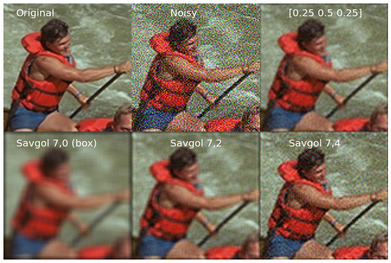
…and it turns out not so much… The main reason is this lack of filtering of the highest frequencies:

…behavior around Nyquist – 40% of the noise and signal is preserved there!

Luckily, there is a way to improve behavior of such filters around Nyquist (by compromising some of the preservations of higher frequencies).

Windowing Savitzky-Golay filters

One of the reasons for not-so-great behavior is use of equal weights for all samples. This is equivalent to applying a rectangular window, and causes “ripples” in frequency domain.

This is similar to applying a “perfect” lowpass filter of sinc and truncating it – which produces undesireable artifacts. Common Lanczos resampling improves it by applying an (also sinc!) window function.

Let’s try the same on the Savitzky-Golay filters. I will use a Hann window (squared cosine), no real reason here, other than “I like it” and I found it useful in some different contexts – overlapped window processing (sums to 1 with fully overlapped windows).

Applying a window here is as easy as simply multiplying the weights by the window function and renormalizing them. Quick visualization of the window function and windowed weights:

Note that window function tends to shrink outer samples strongly towards zero and to get similar behavior, you often need to go with a larger spatial support filter (larger window).

How does it affect the frequency response?

It removes (or at least, reduces) some of the high frequency ripples, but at the same time makes the filter more lowpass (reduces its mid frequency preservation).

Here is how it looks on images:

If you look closely, box-shaped artifacts are gone in the first two of the windowed versions, and are reduced in the 9,6 case.

Savitzky-Golay smoothened gradients

So far I wasn’t super impressed with the Savitzky-Golay filters (for my use-cases) without windowing, but then I started to read more about their typical use – producing smoothened signal gradients / derivatives.

I have written about image (and discrete signal in general) gradients a while ago and if you read my post… it’s not a trivial task at all. Lots of techniques with different trade-offs, lots of maths and physics connections, and somehow any solution I picked it felt like a messy compromise.

The idea of Savitzky-Golay gradients is kind of brilliant – to compute the derivative at a given point, just compute the derivative of the fitted polynomial. This is extremely simple and again has a closed formula solution.

Note however that now we definitely care about differences between odd and even polynomial degrees (look at the slope of lines around 0):

The derivative at 0 can have even an opposite sign between degrees of 2 vs 3 and 4 vs 5.

Since we get the convolution coefficients, we can also plot the frequency responses:

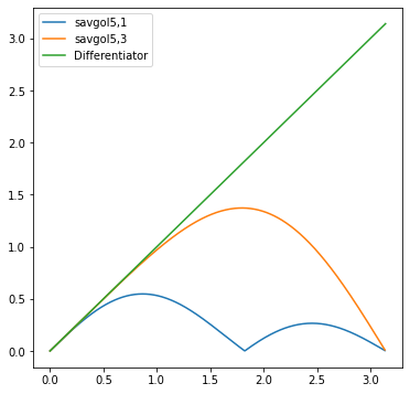
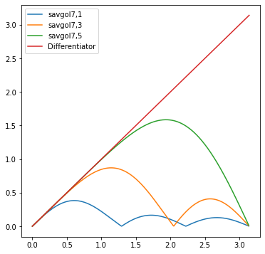
That’s definitely interesting and potentially useful with the higher degrees.

And it’s a neat mental concept (differentiating a continuous reconstruction of the discrete signal) and something I definitely might get back to.

Summary – smoothing filter recommendations

Note: this section is entirely subjective!

After playing a bit with the Savitzky-Golay filters, I personally wouldn’t have a lot of use for them for smoothing digital sample sequences (your mileage may vary).

For preserving edges and not rounding corners, it’s probably best to go with some non-linear filtering – from a simple bilateral, anisotropic diffusion, to Wiener filtering in wavelet or frequency domain.

When edge preservation is less important than just generic smoothing, I personally go with Gaussian-like filters (like the mentioned binomial filter) for their simplicity, trivial implementation, very compact spatial support. Or you could use some proper windowed filter tailored for your desired smoothing properties (you might consider windowed Savitzky-Golay).

I generally prefer to not use exponential moving average filters: a) they are kind of the worst when it comes to preserving mid and lower frequencies b) they are causal and always delay your signal / shift the image, unless you run it forwards and then backwards in time. Use them if you “have to” – like the classic use in temporal anti-aliasing where memory is an issue and storing (and fetching / interpolating) more than one past framebuffer becomes prohibitively expensive. There are obviously some other excellent IIR filters though, even for images – like Domain Transform, just not the exponential moving average.

On the other hand, the application of Savitzky-Golay filters to producing smoothened / “denoised” signal gradients was a bit of an eye opener to me and something I’ll definitely consider the next time I play with gradients of noisy signals. The concept of reconstructing a continuous signal in a simple form, and then doing something with the continuous representation is super powerful and I realized it’s something we explicitly used for our multi-frame super-resolution paper as well.