This post summarizes some thoughts and experiments on “filtering aware image filtering” I’ve been doing for a while.

The core idea is simple – if you have some “fixed” step at the end of the pipeline that you cannot control (for any reason – from performance to something as simple as someone else “owning” it), you can compensate for its shortcomings with a preprocessing step that you control/own.

I will focus here on the upsampling -> if we know the final display medium, or an upsampling function used for your image or texture, you can optimize your downsampling or pre-filtering step to compensate for some of the shortcomings of the upsampling function.

Namely – if we know that the image will be upsampled 2x with a simple bilinear filter, can we optimize the earlier, downsampling operation to provide a better reconstruction?

Related ideas

What I’m proposing is nothing new – others have touched upon those before.

In the image processing domain, I’d recommend two reads. One is “generalized sampling”, a massive framework by Nehab and Hoppe. It’s very impressive set of ideas, but a difficult read (at least for me) and an idea that hasn’t been popularized more, but probably should.

The second one is a blog post by Christian Schüler, introducing compensation for the screen display (and “reconstruction filter”). Christian mentioned this on twitter and I was surprised I have never heard of it (while it makes lots of sense!).

There were also some other graphics folks exploring related ideas of pre-computing/pre-filtering for approximation (or solution to) a more complicated problem using just bilinear sampler. Mirko Salm has demonstrated in a shadertoy a single sample bicubic interpolation, while Giliam de Carpentier invented/discovered a smart scheme for fast Catmul-Rom interpolation.

As usual with anything that touches upon signal processing, there are many more audio related practices (not surprisingly – telecommunication and sending audio signals were solved by clever engineering and mathematical frameworks for many more decades than image processing and digital display that arguably started to crystalize only in the 1980s!). I’m not an expert on those, but have recently read about Dolby A/Dolby B and thought it was very clever (and surprisingly sophisticated!) technology related to strong pre-processing of signals stored on tape for much better quality. Similarly, there’s a concept of emphasis / de-emphasis EQ, used for example for vinyl records that struggle with encoding high magnitude low frequencies.

Edit: Twitter is the best reviewing venue, as I learned about two related publications. One is a research paper from Josiah Manson and Scott Schaefer looking at the same problem, but specifically for mip-mapping and using (expensive) direct least squares solves, and the other one is a post from Charles Bloom wondering about “inverting box sampling”.

Problem with upsampling and downsampling filters

I have written before about image upsampling and downsampling, as well as bilinear filtering.

I recommend those reads as a refresher or a prerequisite, but I’ll do a blazing fast recap. If something seems unclear or rushed, please check my past post on up/downsampling.

I’m going to assume here that we’re using “even” filters – standard convention for most GPU operations.

Downsampling – recap

A “Perfect” downsampling filter according to signal processing would remove all frequencies above the new (downsampled) Nyquist before decimating the signal, while keeping all the frequencies below it unchanged. This is necessary to avoid aliasing.

Its frequency response would look something like this:

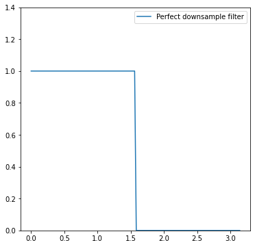
If we fail to anti-alias before decimating, we end up with false frequencies and visual artifacts in the downsampled image. In practice, we cannot obtain a perfect downsampling filter – and arguably would not want to. A “perfect” filter from the signal processing perspective has an infinite spatial support, causes ringing, overshooting, and cannot be practically implemented. Instead of it, we typically weigh some of the trade-offs like aliasing, sharpness, ringing and pick a compromise filter based on those. Good choices are some variants of bicubic (efficient to implement, flexible parameters) or Lanczos (windowed sinc) filters. I cannot praise highly enough seminal paper by Mitchell and Netravali about those trade-offs in image resampling.

Usually when talking about image downsampling in computer graphics, the often selected filter is bilinear / box filter (why are those the same for the 2x downsampling with even filters case? see my previous blog post). It is pretty bad in terms of all the metrics, see the frequency response:

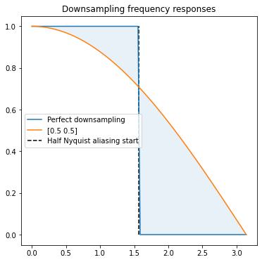
It has both aliasing (area to the right of half Nyquist), as well as significant blurring (area between the orange and blue lines to the left of half Nyquist).

Upsampling – recap

Interestingly, a perfect “linear” upsampling filter has exactly the same properties!

Upsampling can be seen as zero insertion between replicated samples, followed by some filtering. Zero-insertion squeezes the frequency content, and “duplicates” it due to aliasing.

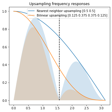
When we filter it, we want to remove all the new, unnecessary frequencies – ones that were not present in the source. Note that the nearest neighbor filter is the same as zero-insertion followed by filtering with a [1, 1] convolution (check for yourself – this is very important!).

Nearest neighbor filter is pretty bad and leaves lots of frequencies unchanged.

A classic GPU bilinear upsampling filter is the same as a filter: [0.125, 0.375, 0.375, 0.125] and it removes some of the aliasing, but also is strong over blurring filter:

We could go into how to design a better upsampler, go back to the classic literature, and even explore non-linear, adaptive upsampling.

But instead we’re going to assume we have to deal and live with this rather poor filter. Can we do something about its properties?

Downsampling followed by upsampling

Before I describe the proposed method, let’s have a look at what happens when we apply a poor downsampling filter and follow it by a poor upsampling filter. We will get even more overblurring, while still getting remaining aliasing:

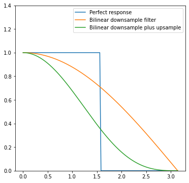
This is not just a theoretical problem. The blurring and loss of frequencies on the left of the plot is brutal!

You can verify it easily looking at a picture as compared to downsampled, and then upsampled version of it:

In motion it gets even worse (some aliasing and “wobbling”):

Compensating for the upsampling filter – direct optimization

Before investigating some more sophisticated filters, let’s start with a simple experiment.

Let’s say we want to store an image at half resolution, but would like it to be as close as possible to the original after upsampling with a bilinear filter.

We can simply directly solve for the best low resolution image:

Unknown – low resolution pixels. Operation – upsampling. Target – original full resolution pixels.  The goal – to have them be as close as possible to each other.

We can solve this directly, as it’s just a linear least squares. Instead I will run an optimization (mostly because of how easy it is to do in Jax! 🙂 ). I have described how one can optimize a filter – optimizing separable filters for desirable shape / properties – and we’re going to use the same technique.

This is obviously super slow (and optimization is done per image!), but has an advantage of being data dependent. We don’t need to worry about aliasing – depending on presence or lack of some frequencies in an area, we might not need to preserve them at all, or not care for the aliasing – and the solution will take this into account. Conversely, some others might be dominating in some areas and more important for preservation. How does that work visually?

This looks significantly better and closer – not surprising, bilinear downsampling is pretty bad. But what’s kind of surprising is that with Lanczos3, it is very similar by comparison:

It’s less aliased, but the results are very close to using bilinear downsampling (albeit with less aliased edges), that might be surprising, but consider how poor and soft is the bilinear upsampling filter – it just blurs out most of the frequencies.

Optimizing (or directly solving) for the upsampling filter is definitely much better. But it’s not a very practical option. Can we compensate for the upsampling filter flaws with pre-filtering?

Compensating for the upsampling filter with pre-filtering of the lower resolution image

We can try to find a filter that simply “inverts” the upsampling filter frequency response. We would like a combination of those two to become a perfect lowpass filter. Note that in this approach, in general we don’t know anything about how the image was generated, or in our case – the downsampling function. We are just designing a “generic” prefilter to compensate for the effects of upsampling. I went with Lanczos4 for the used examples to get to a very high quality – but I’m not using this knowledge.

We will look for an odd (not phase shifting) filter that concatenated with its mirror and multiplied by the frequency response of the bilinear upsampling produces a response close to an ideal lowpass filter.

We start with an “identity” upsampler with flat frequency response. It combined with the bilinear upsampler, yields the same frequency response:

However, if we run optimization, we get a filter with a response:

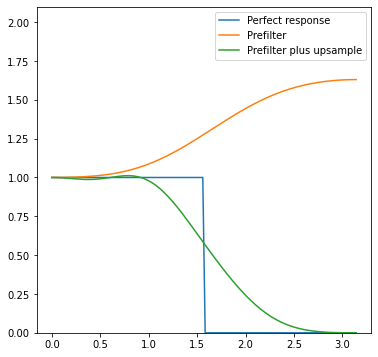
The filter coefficients are…

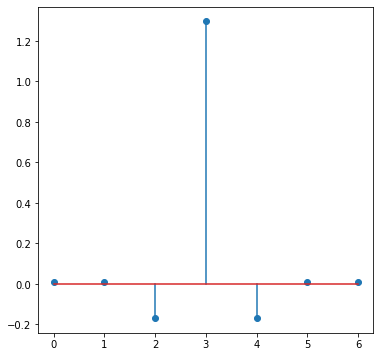
Yes, that’s a super simple unsharp mask! You can safely ignore the extra samples and go with a [-0.175, 1.35, -0.175] filter.

I was very surprised by this result at first. But then I realized it’s not as surprising – as it compensates for the bilinear tent-like weights.

Something rings a bell… sharpening mip-maps… Does it sound familiar? I will come back to this in one of the later sections!

When we evaluate it on the test image, we get:

However if we compare against our “optimized” image, we can see a pretty large contrast and sharpness difference:

The main reason for this (apart from local adaptation and being aliasing aware) is that we don’t know anything about downsampling function and the original frequency content.

But we can design them jointly.

Compensating for the upsampling filter – downsample

We can optimize for the frequency response of the whole system – optimize the downsampling filter for the subsequent bilinear upsampling. 

This is a bit more involved here, as we have to model steps of:

1. Compute response of the lowpass filter we want to model <- this is the step where we insert variables to optimize. The variables are filter coefficients.
2. Aliasing of this frequency response due to decimation.
3. Replication of the spectrum during the zero-insertion.
4. Applying a fixed, upsampling filter of [0.125, 0.375, 0.375, 0.125].
5. Computing loss against a perfect frequency response.

I will not describe all the details of steps 2 and 3 here -> I’ll probably write some more about it in the future. It’s called multirate signal processing.

Step 4. is relatively simple – a multiplication of the frequency response.

For step 5., our “perfect” target frequency response would be similar to a perfect response of an upsampling filter – but note that here we also include the effects of downsampling and its aliasing. We also add a loss term to prevent aliasing (try to zero out frequencies above half Nyquist).

For step 1, I decided on an 8 tap, symmetric filter. This gives us effectively just 3 degrees of freedom – as the filter has to normalize to 1.0. Basically, it becomes a form of [a, b, c, 0.5-(a+b+c), 0.5-(a+b+c), c, b, a]. Computing frequency response of symmetric discrete time filters is pretty easy and also signal processing 101, I’ll probably post some colab later.

As typically with optimization, the choice of initialization is crucial. I picked our “poor” bilinear filter, looking for a way to optimize it.

Without further ado, this is the combined frequency response before:

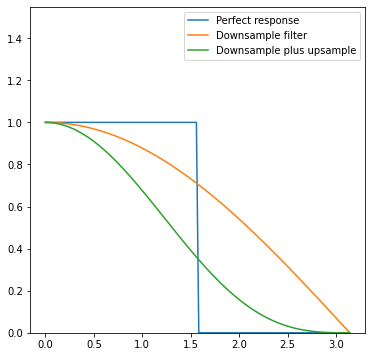
And this is it after:

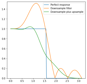
The green curve looks pretty good! There is small ripple, and some highest frequency loss, but this is expected. There is also some aliasing left, but it’s actually better than with the bilinear filter. 

Let’s compare the effect on the upsampled image:

I looked so far at the “combined” response, but it’s insightful to look again, but focusing on just the downsampling filter:

Notice relatively strong mid-high frequency boost (this bump above 1.0) – this is to “undo” the subsequent too strong lowpass filtering of the upsampling filter. It’s kind of similar to sharpening before!

At the same time, if we compare it to the sharpening solution:

We can observe more sharpness and contrast preserved (also some more “ringing”, but it was also present in the original image, so doesn’t bother me as much).

Different coefficient count

We can optimize for different filter sizes. Does this matter in practice? Yes, up to some extent:

I can see the difference up to 10 taps (which is relatively a lot). But I think the quality is pretty good with 6 or 8 taps, 10 if I there is some more computational budget (more on this later).

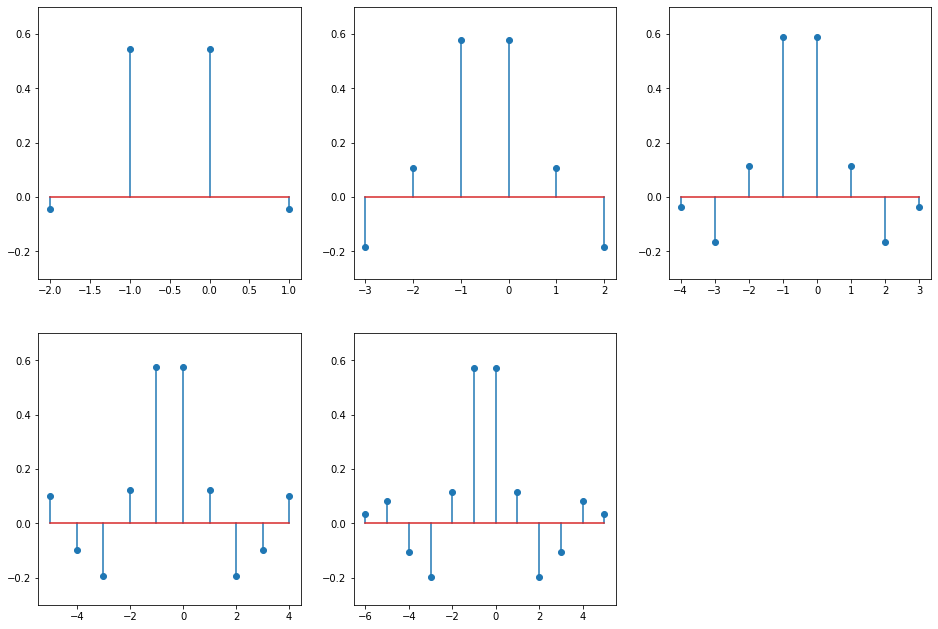
If you’re curious, this is how coefficients look like on plots:

Efficient implementation

You might wonder about the efficiency of the implementation. 1D filter of 10 taps means… 100 taps in 2D! Luckily, proposed filters are completely separable. This means you can downsample in 1D, and then in 2D. But 10 samples is still a lot.

Luckily, we can use an old bilinear sampling trick.

When we have two adjacent samples of the same sign, we can combine them together and in the above plots, turn the first filter into a 3-tap one, the second one into 4 taps, third one into an impressive 4, then 6, and also 6.

I’ll describe quickly how it works.

If we have two samples with offsets -1 and -2 and the same weights of 1.0, we can instead take a single bilinear tap in between those – offset of -1.5, and weight of 2.0. Bilinear weighting distributes this evenly between sample contributions.

When the weights are uneven, it still is w_a + w_b total weight, but the offset between those is w_a / (w_a + w_b).

Here are the optimized filters:

[(-2, -0.044), (-0.5, 1.088), (1, -0.044)]
[(-3, -0.185), (-1.846, 0.685), (0.846, 0.685), (2, -0.185)]
[(-3.824, -0.202), (-1.837, 0.702), (0.837, 0.702), (2.824, -0.202)]
[(-5, 0.099), (-3.663, -0.293), (-1.826, 0.694), (0.826, 0.694), (2.663, -0.293), (4, 0.099)]
[(-5.698, 0.115), (-3.652, -0.304), (-1.831, 0.689), (0.83, 0.689), (2.651, -0.304), (4.698, 0.115)]

I think this makes this technique practical – especially with separable filtering.

Sharpen on mip maps?

One thing that occurred to me during those experiments was the relationship between a downsampling filter that performs some strong sharpening, sharpening of the downsampled images, and some discussion that I’ve had and seen many times.

This is not just close, but identical to… a common practice suggested by video game artists at some studios I worked at – if they had an option of manually editing mip-maps, sometimes artists would manually sharpen mip maps in Photoshop. Similarly, they would request such an option to be applied directly in the engine.

Being a junior and excited programmer, I would eagerly accept any feature request like this. 🙂 Later when I got grumpy, I thought it’s completely wrong – messing with trilinear interpolation, as well as being wrong from signal processing perspective.

Turns out, like with many many practices – artists have a great intuition and this solution kind of makes sense.

I would still discourage it and prefer the downsampling solution I proposed in this post. Why? Commonly used box filter is a poor downsampling filter. Applying sharpening onto it enhances any kind of aliasing (as more frequencies will tend to alias as higher ones), so can have a bad effect on some content. Still, I find it fascinating and will keep repeating that artists’ intuition about something being “wrong” is typically right! (Even if some proposed solutions are “hacks” or not perfect – they are typically in the right direction).

Summary

I described a few potential approaches to address having your content processed by “bad” upsampling filtering, like a common bilinear filter: an (expensive) solution inverting the upsampling operation on the pixels (if you know the “ground truth”), simple sharpening of low resolution images, or a “smarter” downsampling filter that can compensate for the effect that worse upsampling might have on content.

I think it’s suitable for mip-maps, offline content generation, but also… image pyramids. This might be topic for another post though.

You might wonder if it wouldn’t be better to just improve the upsampling filter if you can have control over it? I’d say that changing the downsampler is typically faster / more optimal than changing the upsampler. Less pixels need to be computed, it can be done offline, upsampling can use the hardware bilinear sampler directly, and in the case of complicated, multi-stage pipelines, data dependencies can be reduced.

I have a feeling I’ll come back to the topics of downsampling and upsampling. 🙂