In this post I come back to something I didn’t expect coming back to – dimensionality reduction and compression for whole material texture sets (as opposed to single textures) – a significantly underexplored topic.

In one of my past posts I described how the most simple linear correlation can be used to significantly reduce material texture set dimensionality, and in another one ventured further into a fascinating field of dictionary and sparse compression.

This time, I will describe how we can abandon the land of simple linear correlation (that we explored through the use of SVD) and use data-driven techniques (machine learning!) to discover non-linear functions – using differentiable programming / neural networks.

I’m going to cover:

• Using non-linear decoding on per-pixel data to get better dimensionality reduction than with linear correlation / PCA,
• Augmenting non-linear decoders with neighborhood information to improve the reconstruction quality,
• Using non-linear encoders on the SVD data for target platform/performance scaling,
• Possibility of using learned encoders/decoders for GBuffer data.

Note: There is nothing magic or “neural” (and for sure not any damn AI!) about it, just non-linear relationships, and I absolutely hate that naming.

On the other hand, it does use neural networks, so investors, take notice!

Edit: I have added some example code for this post on github/colab. It’s very messy and not documented, so use at your own responsibility (preferably with a GPU colab instance)!

Inspiration

There have been a few papers recently that have changed the way I think about dimensionality reduction specifically for representing materials and how the design space might look like.

I won’t list all here, but here (and here or here) are some more recent ones that stood out and I remembered off the top of my head. The thing I thought was interesting, different, and original was the concept of “neural deferred rendering” – having compact latent codes that are used for approximating functions like BRDFs (or even final pixel directional radiance) expanded by a tiny neural network, often in the form of a multi-layer perceptron.

What if we used this, but in a semi-offline setting? 

What if we used tiny neural networks to decode materials?

To explain why I thought it could be interesting to bother to use a “wasteful” NN (NNs are always wasteful due to overcompleteness, even if tiny!), let’s start with function approximation and fitting using non-linear relationships.

Linear vs non-linear relationships

In my post about SVD and PCA, I discussed how linear correlation works and how it can be used. If you haven’t read my post, I recommend to pause reading this one, as I will use the same terminology, problem setting, and will go pretty fast.

It’s an extremely powerful relationship; and it works so well because many problems are linear once you “zoom in enough” – the principle behind truncated Taylor series approximations. Local line equations rule the engineering world! (And can be used as an often more desirable replacement for the joint bilateral filter).

So in the case of PCA material compression, we assume there is a linear relationship between the material properties and color channels and use it to decorrelate the input data. Then. we can ignore the components that are less correlated and contribute less, reducing the representation and storage to just a few channels.

Then the output can be computed by a weighted combination of adding them together.

Unfortunately, once we “zoom out” of local approximations (or basically look at most real world data), relationships in the data stop being so “linear”.

Often PCA is not enough. Like in the above example – we discard lots of useful distinction between some points.

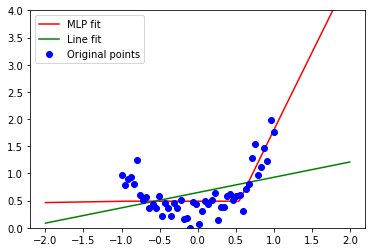
But let’s go back and have a look at a different set of simple observations(represented as noisy data points on axis x and y):

A linear correlation cannot capture much of the distribution shape and is very lossy. We can guess why – because this looks like a good old parabola, a quadratic function.

Line fit is not enough and errors are large both “inside” the set, as well as approaching its ends.

This is what drove the further developments of the field of machine learning (note: PCA is definitely also a machine learning algorithm!) – to discover, explain, and approximate such growingly more complex relationships, with both parametric (where we assume some model of reality and try to find the best parameters), as well as non-parametric (where we don’t formulate the model of reality or data distribution) models.

The goal of Machine Learning is to give reasonable answers where we simply don’t know the answers ourselves – when we don’t have precise models of reality, there are too many dimensions, relationships are way too complex, or we know they might be changing.

In this case, we can use many algorithms, but the hottest one are “obviously” neural networks. 🙂 The next section will try to look at why, but first let’s approximate our data with a small, few neurons in a hidden layer Mult-Layer Perceptron NN with a ReLU activation function (ReLU is a fancy name for max(x, 0) – probably the simplest non-linear function that is actually useful and differentiable almost everywhere!) with 3 hidden neurons:

Or for example with 4 neurons as:

If we’re “lucky” (good initialization), we could get a fit like this:

It’s not “perfect”, but much better than the linear model. SVD, PCA, or line fits in a vanilla form can discover only linear relationships, while networks can discover some other, interesting nonlinear ones.

And this is why we’re going to use them!

Digression – why MLP, ReLU, and neural networks are so “hot”?

A few more words on the selected “architecture” – we’re going to use a most old-school, classic Neural Network algorithm – Multilayer Perceptron.

When I first heard about “Neural Networks” at college around the mid 00s, in the introductory courses, “neural networks” were almost always MLPs and considered quite outdated. I also learned about Convolutional Networks and implemented one for my final project, but those were considered slow, impractical, and generally worse performing than SVMs and other techniques – isn’t it funny how things change and history turns around? 🙂

Why are neural networks used today everywhere and for almost everything?

There are numerous explanations, from deeply theoretical ones about “universal function approximation”, through hardware based ones (efficient to execute on GPUs, but also HW accelerators being built for those), but for me the most both pragmatic, as well as perhaps a bit cynical is – a circular explanation – because the field is so “hot” that a) actual research went into building great tools and libraries for those, plus b) there is a lot of know-how.

It’s super trivial to use a neural network to solve a problem where you have “some” data, the libraries and tooling are excellent, and over a decade of recent research (based on half a century of fundamental research before that!) went into making them fast and well understood.

MLP with a ReLU activation provides piecewise linear approximations to the actual solutions. In our example, they will never be able to learn a real parabola, but given enough data it can perform very well if we evaluate on the same data.

While it doesn’t make sense to use NNs for data that we know is drawn from a small parabola (because we can use a parametric model – both more accurate, as well as way more efficient), if we had more than three a few dimensions or a few hundred samples, human reasoning, intuition and “eyeballing” starts to break down.

The volume space of possible solutions increases exponentially (“curse of dimensionality”). For the use-case we’ll look at next (neural decompression of textures), we cannot just quickly look at the data and realize “ok, there is a cubic relationship in some latent space between the albedo and glossiness”- so finding those with small MLPs is an attractive alternative.

But it can very easily overfit (fail to discover real, underlying relationship in the data – variance bias trade-off); for example increasing the hidden layer neuron count to 256, we can get:

Luckily, for our use-case – it doesn’t matter. For compressing fixed data, the more over-fitting, the better! 🙂 

Non-linear relationships in textures

With the SVD compressed example, we were looking at N input channels (stored in textures), with K (9 in the example we analyzed) output channels, with each output channel given by x_0 * w_0 + … + x_n-1 w_n-1, so a simple linear relationship.

Let’s have a look again at N input channels, K output channels, but in between them a single hidden layer of 64 neurons with a ReLU function:

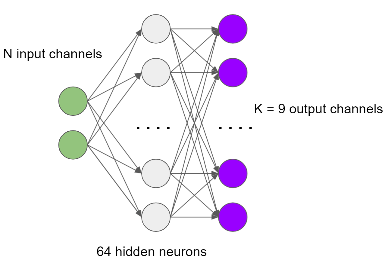
This time, we perform a matrix multiplication (or a series of multiply-adds) for every neuron in the hidden layer and use those intermediate, locally computed values as our “temporary” input channels that get fed to a final matrix multiplication producing the output.

This is not a convolutional network. The data still stays “local”, we read same amount of information per channel. During network training, we are training both the network, as well as the input compressed texture channels.

If those terms don’t mean much to you, unfortunately I won’t go much deeper into how to train a network, what optimizers and learning rates to use (I used ADAM with learning rate of 0.01) etc. – there are people who are much more competent and explain it much better. I learned from the Deep Learning book and can recommend it, a clear exposition to both theory and some practice, but it was a while ago, so maybe better resources are available now.

I did however write about optimizing latent codes! About optimizing SVD filters with Jax, optimizing blue noise patterns, and about finding latent codes for dictionary learning. In this case, texture contents are simply a set of variables optimized during network training, also through gradient descent / backpropagation. The whole process is not optimized at all and takes a couple of minutes (but I’m sure could be made much faster).

Without further ado, here’s the numerical quality comparison, number of channels vs PSNR:

When I first saw the numbers and behavior for the very low channel count, I was pretty impressed. The quantitative improvement is significant, over a few db. In the case of 4 channels, it turns it from useless (PSNR below 30dB), to pretty good – over 36dB!

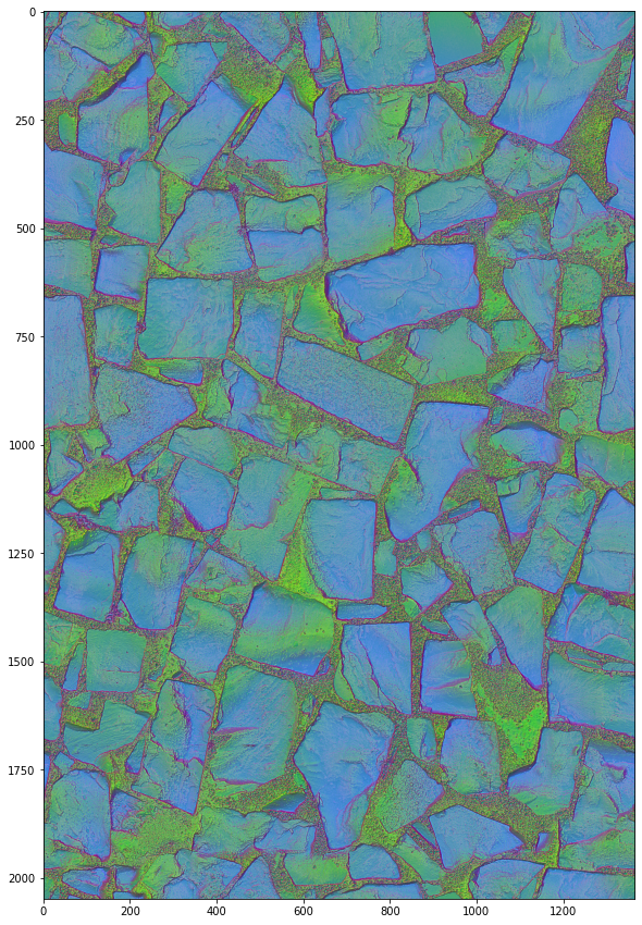
Here’s a visual comparison:

That’s the case where you don’t even need gifs and switching back and forth – the difference is immediately obvious on the normal map as well as the height map (middle). It is comparable (almost exactly the same PSNR as well) to the 5 channels linear encoding.

This is the power of non-linearity – it can express approximations of relationships between the normal map channels like x^2 + y^2 + z^2 = 1, which is impossible to express through a single linear equation.

How do the latent codes look like? Surprisingly similar to PCA data and reasonably uncorrelated, like:

Efficient implementation

Before I go further, how fast / slow would that be in practice? 

I have not measured the performance, but the most straightforward implementation is to compute the per-pixel 64 values, storing them in either registers or LDS through a series of 64×4 MADDs, and then do another 64×9 MADDs to compute the final channels, totaling 832 multiply add ops.

For intermediate channel (64):
  For input channel (1-5):
    Intermediate += Input * weight
    Intermediate = max(0, Intermediate)
For output channel (9):
  For intermediate channel (64):
    Output += Intermediate * weight

This sounds expensive, however all “tricks” of optimizing NNs apply – I’m pretty sure you can use “tensor cores” on nVidia hardware, and very aggressive quantization – not just half floats, but also e.g. 8 or 4 bit smaller types for faster throughput / vectorization.

There’s also a possibility of decompressing this into some intermediate storage / cache like virtual textures, but I’m not sure if this would be beneficial? There’s an idea floating around for at least half a decade about texel shaders and how they could be the solution to this problem, butI’ve been far away from GPU architecture for the past 4 years to not have an opinion on that.

Would this work under bilinear interpolation?

A question that came to my mind was – does this non-linear decoding of data break under linear interpolation (or any linear combination) of the decoded inputs?

I have performed the most trivial test – upscale encoded data bilinearly by 4x, decode, downsample, and compare to the original decoded. It seems to be very close, but this is an empirical experiment on only one example. I am almost sure it’s going to work well on more materials – the reason is how tiny is the network as compared to the number of texels, with not much room to overfit.

To explain this intuition, here is again example from above – where small parameter count and undefitting (left) behaves well between the input points, while the overfit case (right) would behave “badly” and non-linearly under linear interpolation:

What if we looked at neighbors / larger neighborhoods?

When you look at material textures, one thing that comes to mind is that per channel correlations might be actually less obvious than another type of correlations – spatial ones.

What I mean here is that some features depend not only on the contents of the single pixel, but much more on where it is and what it represents.

For example – a normal map might represent the derivative / gradient of the height map, and cavity or AO map darker spots be surrounded by heightmap slopes. 

We could use either authored features like gradients, or just general convolution networks and let the network learn those non-linearities, but that could be too slow.

I had another idea that is much simpler/cheaper and seems to work quite ok – why not just look at the blurred version of the texel neighborhood? In the extreme close to zero cost approximation – if we looked at one of the next levels in the mip chain which is already built?

So as an input of the network, I add simulated reading from 2 mip levels down (by downsampling the image 4x, and then upsampling back).

This seems to improve the results quite significantly in this my favorite (strong compression, good PSNR results) 2-5 channel regime:

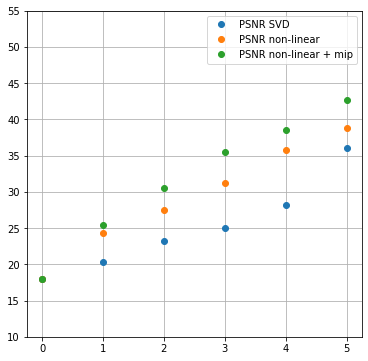
Maybe not as spectacular, but now together with those two changes we’re talking about improving PSNR for storing just 3 channels and reconstructing 9 from 25dB to over 35.5dB, this is a massive improvement!

Why not go ahead with full global encoding and coordinate networks?

Success of recent techniques in neural rendering and computer vision where the input are just spatial coordinates (like brilliant NeRF), begs a question – why not use same approach for compressing materials / textures? My understanding is that a fully trained NeRF actually uses more data than in the input (expansion instead of compression!), but even if we went with a hybrid solution (some latent code + a mixed coordinate and regular input network), for the decoding use on GPUs we’d generally don’t want to have a representation with “global support” (where every piece of information describes the behavior / decoded data in all locations).

If you need to access information about the whole texture to encode every single pixel, the data is not going to fit in the cache… And it doesn’t make sense. I think of it this way – if you were rendering an open world, to render a small object in one place would you want be required to always access information about a different object 3mile / 5km away?

Local support is way more efficient (as you need to read less data that fits in the local cache), and even techniques like JPEG that use global support basis like DCT only per a local, small tile.

Neural decompressor of linear SVD data

This is an idea that occurred to me when playing with adding those spatial relationships. Can a “neural” decompressor learn some meaningful non-linear decoding of linearly encoded data? We could use a learned decoder on fast, linearly encoded data.

This would have two significant benefits:

1. The compression / encoding would be significantly faster.
2. Depending on the speed / performance (or memory availability if caching) of the platform, one could pick either fast, linear decompression, or a neural network to decompress.
3. Artists could iterate on linear, SVD data and have a guarantee that the end result will be higher quality on higher end platforms.

In this set-up, we just freeze the latent code computed through SVD and optimize only the network. The network has access to the SVD latent code and two of the following mip levels.

The results are not as impressive be before, but still getting ~4dB extra from exactly same input data is an interesting and most likely applicable result?

GBuffer storage?

As a final remark, in some cases, small NNs could be used for decoding data stored in GBuffer in the context of deferred shading. If many materials could be stored using the same representation, then decoding could happen just before shading.

This is not as bizarre an idea as it might seem – while compression would most likely be more modest, I see a different benefit – many game engines that use deferred shading have hand-written hard-coded spaghetti code logic for packing different material types and variations with many properties, with equally complicated decoding functions.

When I worked on GoW, I spent weeks on “optimal” packing schemes that were compromising the needs of different artists and different types of materials (anisotropic specular, double specular lobes, thin transmission, retroreflective specular, diffusion with different profiles…).

…and there were different types of encoding/decoding functions like perceptually linearizing roughness, and then converting it to a different representation for the actual BRDF evaluation. Lots of work that was interesting (a fun challenge!) at times, but also laborious, and sometimes heartbreaking (when you have to pick between using more memory and the whole game losing 10% performance, and telling an artist that a feature you wrote for them and they loved will not be supported anymore).

It could be an amazing time saver and offloading for the programmer to rely on automatic decoding instead of such imperfect heuristics.

Summary

In this post, I returned to some ideas related to compressing whole material sets together – and relying on their correlation.

This time, we focused on the assumption of the existence of non-linear relationships in data – and used tiny neural networks to learn this relationship for efficient representation learning and dimensionality reduction. 

My post is far from exhaustive or applicable – it’s more of an idea outline / sketch, and there are a lot of details and gaps to fill – but the idea definitely works! – and provides real, measurable benefit – on the limited example I tried it on. Would I try moving in this direction in production? I don’t know, maybe I’d play more with compressing material sets if I was under dire need for reducing material sizes, but otherwise I’d probably spend some more time following the GBuffer compression automation angle (knowing it might be tricky to make practical – how do you obtain all the data? how do you eveluate).

If there’s a single outcome outside of me again toying with material sets, I hope it somewhat demystified using neural networks for simple data driven tasks:

• It’s all about discovering, non-linear relationships in lots of complicated, multi-dimensional data,
• Despite limitations (like ReLU can provide only a piecewise linear function approximation) they can indeed discover those in practice,
• You don’t need to run a gigantic end-to-end network that has millions of parameters to see benefits of them,
• Small, shallow networks can be useful and fast (832 multiply-adds on limited precision data is most likely practical)!

Edit: I have added some example code for this post on github/colab. It’s very messy and not documented, so use at your own responsibility (preferably with a GPU colab instance)!