In previous part of the mini-series I covered dithering definition and how dithering changes error characteristics of simple 1D quantization and functions.

In this part I will try to look at what blue noise is, but first wanted to have a look at a number sequence that I used in the previous post and I find very useful.

You can find a Mathematica notebook for golden sequence here and its pdf version here.

For the second part of the post you can find the notebook here and its pdf version here.

Golden ratio sequence

In previous post I used “some” quasi-random function / sequence and mentioned that it’s not perfect, but very useful. The sequence is a sequence made of fractional part of next multiplications of a golden number.

FractionalPart[N*GoldenRatio]

I found idea for using it in a paper “Golden Ratio Sequences For Low-Discrepancy Sampling” by Colas Schretter and Leif Kobbelt.

This is incredibly fascinating sequence, as it seems to distribute next values very well and quite far apart:

The differences between next elements are in modulus 1:

{0.381966, 0.618034, 0.381966, 0.381966, 0.618034, 0.381966, 0.618034, 0.381966}

So oscillating golden number modulo 1 itself and 2 minus golden number modulo 1. Both numbers are distant enough from zero and one to produce well-distributed sequence where next samples add lots of information.

Edit: Mikkel Gjøl observed that modulo/toroidal minimum distance of 0.618034 is 0.381966, so the sequence becomes:

{0.381966, 0.381966, 0.381966, 0.381966, 0.381966, 0.381966, 0.381966, 0.381966}

I find it a remarkably beautiful property!

Even for small number of “samples” in the sequence, they cover whole 0-1 range very well:

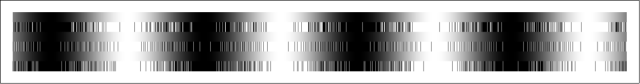
Numbers plotted as colors also look “pleasant”:

If we look at its periodogram:

We also find some fascinating properties. First of all, energy seems to increase with frequencies. There are visible “spikes” in some frequencies and what is even more interesting is that every next spike happens at a frequency that is golden ratio times higher and it has golden ratio times more energy! I don’t have any explanation for it… so if you are better than me at maths, please contribute with a comment!

This frequency characteristic is extremely useful, however doesn’t satisfy all of our dithering needs. Why? Imagine that our source signal that we are dithering contains same frequencies. Then we would see extra aliasing in those frequencies. Any structure in noise used for dithering can become visible, and can produce undesired aliasing.

I still find this sequence extremely valuable and use it heavily in e.g. temporal techniques (as well as hemispherical sampling). There are other very useful low-discrepancy sequences that are heavily used in rendering – I will not cover those here, instead reference the physically based rendering “bible” – “Physically Based Rendering, Third Edition: From Theory to Implementation” by Matt Pharr, Wenzel Jakob and Greg Humphreys and chapter 7 that authors were kind enough to provide for free!

For now let’s look at blue noise and theoretically “perfect” dithering sequences.

Blue noise

What is blue noise? Wikipedia defines it as:

Blue noise is also called azure noise. Blue noise’s power density increases 3 dB per octave with increasing frequency (density proportional to f ) over a finite frequency range. In computer graphics, the term “blue noise” is sometimes used more loosely as any noise with minimal low frequency components and no concentrated spikes in energy.

And we will use here this more liberal definition (with no strict definition of frequency distribution density increase).

We immediately see that previous golden ratio sequence is not blue noise, as it has lots of visible spikes in spectrum. Perfect blue noise has no spikes and therefore is not prone to aliasing / amplifying those frequencies.

There are many algorithms for generating blue noise, unfortunately many of them heavily patented. We will have a look at 2 relatively simple techniques that can be used to approximate blue noise.

Generating blue noise – highpass and remap

The first technique we will have a look at comes from Timothy Lottes and his AMD GPUOpen blog post “Fine art of film grain”.

The technique is simple, but brilliant – in step one let’s take a noise with undesired frequency spectrum and just reshape it by applying high pass filter.

Unfortunately, arbitrary high pass filter will produce a signal with very uneven histogram and completely different value range than original noise distribution:

This is where part 2 of the algorithm comes in. Remapping histogram to force it to be in 0-1 range! Algorithm is simple – sort all elements by value and then remap the value to position in the list.

Effect is much better:

Unfortunately, histogram remapping operation also changes the frequency spectrum. This is inevitable, as histogram remapping changes relative value of elements not linearly. Values in middle of the histogram (corresponding to areas that originally had lost of low frequency component) will be changed much more than values in areas with high frequency content. This way part of high-pass filtering effect is lost:

Still, effect looks pretty good compared to no high pass filtering:

Its frequency spectrum also looks promising:

However, there is still this trailing low pass component. It doesn’t contain lots of energy, but still can introduce some visible low pass error in dithered image…

What we can do is to re-apply the technique again!

This is what we get:

Frequency spectrum definitely looks better and whole algorithm is very cheap so we can apply it as many times as we need.

Unfortunately, no matter how many times we will reapply it, it’s impossible to “fix” all possible problematic spots.

I think about it this way – if some area of the image contains only very low frequency, after applying highpass filter, it will get few adjacent values that are very close to zero. After histogram remapping, they will get remapped to again similar, adjacent values.

It’s possible that using a different high pass filter or adding some noise between iterations or detecting those problematic areas and “fixing” them would help – but it’s beyond scope of this post and the original technique.

What is worth noting is that original algorithm gives sequence that is not perfect, but often “good enough” – it leaves quite bad local spots, but optimizes frequency spectrum globally .Let’s check it in action.

Results

Let’s have a look at our initial, simple 1D dithering for binary quantization:

We can see that both golden ratio sequence and our highpass and remap are better than regular noise. However it seems like golden ratio sequence performs better here due to less “clumping”. You can see though some frequency “beating” corresponding to peak frequencies there:

So this is not a perfect technique, but a) very fast b) tweakable and c) way better than any kind of white noise.

Better? Slower blue noise

Ok, what could we do if we wanted some solution that doesn’t contain those local “clumps”? We can have a look at Siggraph 2016 paper “Blue-noise Dithered Sampling” by Iliyan Georgiev and Marcos Fajardo from Solid Angle.

The algorithm is built around the idea of using probabilistic technique of simulated annealing to globally minimize desired error metric (in this case distance between adjacent elements).

I implemented a simple (not exactly simulated annealing; more like a random walk) and pretty slow version supporting 1, 2 and 3D arrays with wrapping: https://github.com/bartwronski/BlueNoiseGenerator/

As usually with probabilistic global optimization techniques, it can take pretty damn long! I was playing a bit with my naive implementation for 3D arrays and on 3yo MacBook after a night running it converge to at best average quality sequence. However, this post is not about the algorithm itself (which is great and quite simple to implement), but about the dithering and noise.

For the purpose of this post, I generated a 2000 elements, 1D sequence using my implementation.

This is a plot of first 64 elements:

Looks pretty good! No clumping, pretty good distribution.

Frequency spectrum also looks very good and like desired blue noise (almost linear energy increase with frequency)!

If we compare it with frequency spectrum of “highpass and remap”, they are not that different; slightly less very low frequencies and much more of desired very high frequencies:

We can see it compared with all other techniques when applied to 1D signal dithering:

It seems to me to be perceptually best and most uniform (on par with golden ratio sequence).

We can have a look at frequency spectrum of error of those:

If we blur resulting image, it starts to look quite close to original simple sine signal:

If I was to rate them under this constraints / scenario, I would probably use order from best to worst:

• Golden ratio sequence,
• Blue noise generated by Solid Angle technique,
• Blue noise generated by highpass and remap,
• White noise.

But while it may seem that golden ratio sequence is “best”, we also got lucky here, as our error didn’t alias/”resonate” with frequencies present in this sequence, so it wouldn’t be necessarily best case for any scenario.

Summary

In this part of blog post mini-series I mentioned blue noise definition, referenced/presented 2 techniques of generating blue noise and one of many general purpose high-frequency low-discrepancy sampling sequences. This was all still in 1D domain, so in the next post we will have a look at how those principles can be applied to dithering of a quantization of 2D signal – like an image.

Blog post mini-series index.

References

https://www.graphics.rwth-aachen.de/media/papers/jgt.pdf “Golden Ratio Sequences For Low-Discrepancy Sampling”, Colas Schretter and Leif Kobbelt

“Physically Based Rendering, Third Edition: From Theory to Implementation”, Matt Pharr, Wenzel Jakob and Greg Humphreys.

https://en.wikipedia.org/wiki/Colors_of_noise#Blue_noise 

http://gpuopen.com/vdr-follow-up-fine-art-of-film-grain/ “Fine art of film grain”, Timothy Lottes

“Blue-noise Dithered Sampling”, Iliyan Georgiev and Marcos Fajardo