Introduction

I recently read the “Gaussian Blue Noise” paper by Ahmed et al. and was very impressed by the quality of their results and the rigor of their method.

They provide a theoretical framework to analyze the quality of blue noise from a frequency analysis perspective and propose an improved technique for generating blue noise patterns. This use of blue noise is very different from “blue noise masks” and regular dithering – about which I have a whole series of posts if you’re interested.

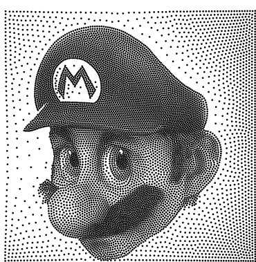
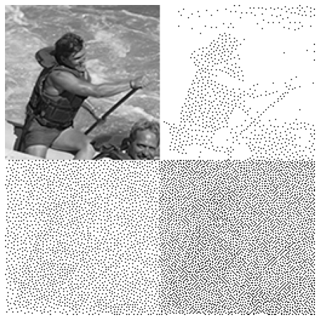
Authors of the GBN paper show some gorgeous blue noise stippling patterns:

Their work is based on an offline optimization procedure and has inspired me to solve a different problem – progressive stippling. I thought it’d look super cool and visually pleasing to have some “progressive” blue-noise stippling animations from an image.

By progressive, we mean creating a set of N sample sets, where:

• each one has 1…N samples, 
• a set K is a subset of the set K+1 (set K+1 adds one more point to the set K),
• each set K fulfills the blue noise criterion.

By fulfilling all three criteria (especially the second), the “quality” (according to the third) of the last complete set cannot be as high as in, for example, the “Gaussian Blue Noise” paper. In optimization, every new constraint and additional requirement sacrifices other requirements.

We won’t have as excellent blue noise properties as in the cited GBN paper, but as we’ll see, we can get “good enough” and visually pleasing results.

Progressive sampling is a commonly used technique in Monte Carlo rendering for reconstruction that improves over time (critical in real-time/interactive applications) but less commonly in stippling/dithering – I haven’t found a single reference to progressive stippling.

Here, I propose a straightforward method to achieve this goal.

Method

As a method, I augment my “simplified” variation of the greedy void and cluster algorithm with a trivial modification to the initial “energy” potential field.

Instead of uniform initialization, I initialize it with the image intensity scaled by some factor “a.”

(Depending on the type of stippling, with black “ink” dots or with the bright “light splats,” you might want to “negate” this initialization)

Factor “a” will balance the image content’s importance compared to filling the whole image plane with the blue noise distribution property.

In my original implementation, the Gaussian kernel used for energy modification was unnormalized and didn’t include a correction for small sigma. I fixed those to allow for easier experimentation with different spatial sigmas.

One should consider the boundary conditions for applying the energy modification function (zero, mirror, clamp) for the desired behavior. For example, spherically-wrapped images like environment maps should use “wrap” while displayable ones might want to use “clamp.” I ignore it here and use the original “wrap” formulation, suitable for use cases like spherical images.

We stop the iteration after we reach the desired point count – for example, equal to the average brightness of the original image.

This is the whole method!

Here is the complete code:

def gauss_small_sigma(x: np.ndarray, sigma: float):
    p1 = scipy.special.erf((x - 0.5) / sigma * np.sqrt(0.5))
    p2 = scipy.special.erf((x + 0.5) / sigma * np.sqrt(0.5))
    return (p2 - p1) / 2.0
 
 
def void_and_cluster(
    input_img: np.ndarray,
    percentage: float = 0.33,
    sigma: float = 0.9,
    content_bias: float = 0.5,
    negate: bool = False,
) -> Tuple[np.ndarray, np.ndarray]:
    size = input_img.shape[0]
 
    wrapped_pattern = np.hstack((np.linspace(0, size / 2 - 1, size // 2), np.linspace(size / 2, 1, size // 2)))
    wrapped_pattern = gauss_small_sigma(wrapped_pattern, sigma)
    wrapped_pattern = np.outer(wrapped_pattern, wrapped_pattern)
    wrapped_pattern[0, 0] = np.inf
 
    lut = jnp.array(wrapped_pattern)
    jax.device_put(lut)
 
    def energy(pos_xy_source):
        return jnp.roll(lut, shift=(pos_xy_source[0], pos_xy_source[1]), axis=(0, 1))
 
    points_set = []
 
    energy_current = jnp.array(input_img) * content_bias * (-1.0 if negate else 1.0)
    jax.device_put(energy_current)
 
    @jax.jit
    def update_step(energy_current):
        pos_flat = energy_current.argmin()
        pos_x, pos_y = pos_flat // size, pos_flat % size
        e = energy_current[pos_x, pos_y]
        return energy_current + energy((pos_x, pos_y)), pos_x, pos_y, e
 
    final_stipple = np.zeros_like(lut) if negate else np.ones_like(lut)
 
    samples = []
    for x in range(int(input_img.size * percentage)):
        energy_current, pos_x, pos_y, e = update_step(energy_current)
        samples.append((pos_x, pos_y, input_img[pos_x, pos_y]))
        final_stipple[pos_x, pos_y] = 1.0 if negate else 0.0
    return final_stipple, np.array(samples)

And it works pretty well:

With different factors “a,” we get the different balancing of filling the overall image space more as contrasted to a higher degree of importance sampling with the equal sample count:

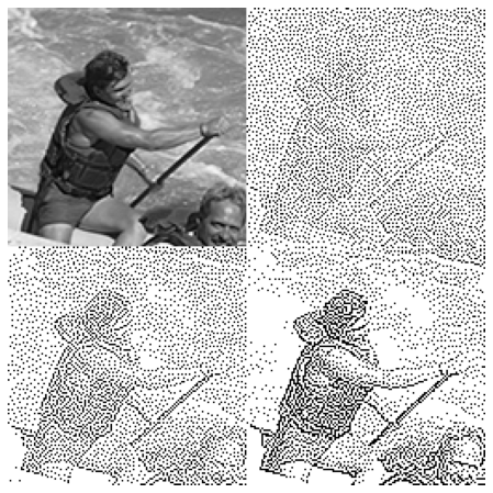
When the parameter goes towards infinity, we get the pure progressive sampling of the original image. The other extreme will produce pure blue noise, filling space and ignoring the image content:

The behavior of low values is interesting. With the increasing point count, they first reveal the shape, then give a ghostly “hint” of the shape underneath, and finally turn into almost uniform spatial filling:

Why does this work?

Results look pretty remarkable, given the straightforward and almost “minimal” method, so why does it work? 

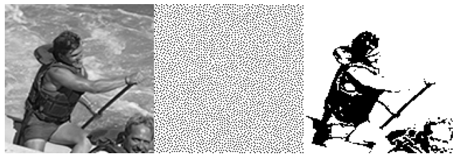
When we initialize the energy field with the image, we find the brightest/darkest point (depending on whether we negated the image content) as the one with minimum energy. After the first update, we add energy to this position. The next iteration finds and updates a different point. Here is a visualization (slightly exaggerated) for 1, 2, 11, and 71 points:

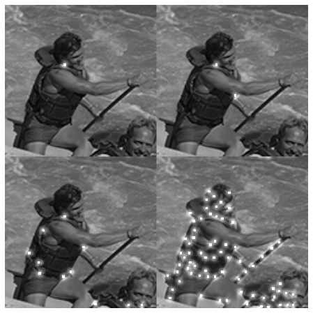
Each iteration both excludes the point from being reprocessed (sets it as “infinite energy”) as well as produces a Gaussian “splat” that makes the points around it less desirable to be “picked” in the following close iterations. The algorithm will choose something further away from it. The “a” constant and the Gaussian sigma balance the repulsion of points with the priority of the pixel intensity.

Edge sampling

When stippling, classic literature (ref1 ref2) emphasizes how the stippling of the edges is more critical than stippling the constant areas – both for “artistic” reasons and because the human visual system has strong edge detection mechanisms.

The above example worked very well for two reasons.

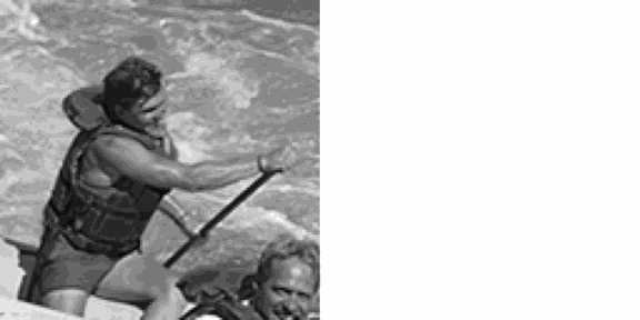
The most important secret was that Kodak images – like most images on the internet – are sharpened for display and printing. If you look at the boat paddle in the picture, you will notice a bright halo around it. Almost all images have sharpening, tiny halos, and gradient reversals.

The second reason relates to the method: looking at single points in combination with blue noise like “repulsion” will push many points to the edges.

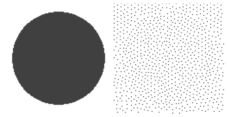
But if we look at the simplest analytical unsharpened example – a circle, we find that the shape is somewhat visible, but not overly so:

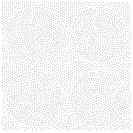
The solution is straightforward, and along the lines of observation of sharpened internet images, we can pre-sharpen the image arbitrarily (just before generating the initialization energy).

The amount of sharpening determines how strong we are going to reproduce the edges:

All of the above are very usable, and I like it the most and find it the most useful when our constant “a” is low (biasing the results towards preserving space-filling blue-noise properties more than contents brightness). Visible edges can make a huge difference in how we perceive low-contrast shapes.

Improving the final state further

The suboptimality of the described method at the final state can be improved slightly (at the cost of breaking the progressive results) by “fine-tuning” the positions of points based on the last point set and according to the energy defined like in the GBN paper. However, one would have to allow it not to go too far from the original positions to preserve the progressive property.

This approach is not unlike standard methods in deep learning, where one fine-tunes the training/optimization results on specific, more relevant examples – typically using fewer iterations and a slower learning rate to avoid over-fitting.

Use for importance sampling

The use-case I have described so far is… cute and produces fun and pretty animations, but can it be useful? Probably the concept of “progressive stippling” – not so much beyond artistic expression.

But if we squint our eyes, we make the following observations:

1. Thanks to the “progressive” property, points are sorted according to “importance,”
2. Importance consists of two components:
   1. Blue noise spatial distribution,
   2. The value of the input pixel.
3. We don’t have to stop at the average brightness and can continue until we fill all the points.

Note, however, that the sorting/importance is not according to just the brightness or good spatial distribution; it’s a hybrid metric that combines both and depends on the spatial relationships and distribution.

Could we use it for blue noise distributed importance sampling of images?

Importance sampling of images is commonly used for evaluating image-based lighting or sampling 2D look-up tables for terms we lack analytical solutions. Most approaches rely on complicated spatial division structures built offline and traversed during the sampling process.

I propose to use the sorted progressive stippling points (and their pixel values) in the importance sampling process.

Let’s use a different Kodak image, a crop of the lighthouse (and inverting for the sampling of the brights):

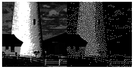
If we plot the brightness of the consecutive points in the sequence, we observe it is a very “noisy” version and distorted version of the image histogram:

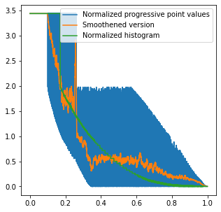
The distortion is non-obvious, hard to predict, and depends on the spatial co-locality of the points in the image. Different images with identical histograms will get different results based on where the similarly valued pixels are.

To use it in practice for importance sampling, I propose to use a smoothened, normalized version of this histogram as a PDF. Based on the inverse-sampled value, pick a point from the sequence. The sample stores information about its intensity and the original location in the image. 

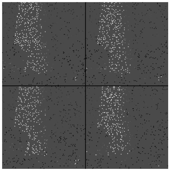
For simplicity’s sake and a quick demonstration, I will use an ad-hoc inverse CDF of exponentiating a random number to the power of 3 (equivalent to $\frac{1}{3x^{\frac{2}{3}}} PDF).

For example, with the uniform random variable value of 0.1, we will pick 0.1**3 == 0.001 percentile point from the progressive stippling sequence.

The following figure presents what the four different batches of 1000 random samples from this distribution look like:

And by comparison, the same sample counts, but with pure importance sampling based on the image brightness:

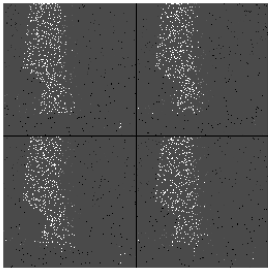
The latter has significantly more “clumping” and worse space coverage outside bright regions. This difference might matter for the cases of significant mismatch of the complete integrand (often a product of multiple terms) with the image content.

Many small details are necessary to make this method practical for Monte Carlo integration. A pixel’s fixed (x, y) position is not enough to sample other terms appearing in an actual Monte Carlo integral, like a continuous PDF of a BRDF. One obvious solution would be to perform jittering within pixel extents based on additional random variables.

I don’t test the effectiveness of this method. I believe it would give less variance at low sample counts but not improve the convergence (this is typical with blue noise sampling).

Finally, this method can be expanded to more than just two dimensions – as long as we have a discrete domain and can splat samples into it.

But I leave all of the above – and evaluation of the efficacy of this method to the curious reader.

Conclusions

I have presented an original problem – progressive stippling of images and a method to compute it with a few lines of code of modification of the “void and cluster” blue noise generation method.

It worked surprisingly well, and I consider it a fun, successful experiment, just look again at those animations:

It seems to have some applications beyond fun animations, like very fast blue-noise preserving importance sampling of textures, environment maps, and look-up tables. I hope it inspires some readers to experiment with that use case.