Introduction

This will be a blog post that is second in an (unanticipated) series on interesting uses of the JAX numpy autodifferentiation library, as well as an extra post in my very old post series on dithering in games and blue noise specifically.

I am going to describe how we can use auto-differentiation and loss function optimization to perform a precomputation of a dithering pattern directly with a desired Fourier/frequency spectrum and the desired range of covered values by backpropagating through those two (differentiable!) transforms.

While I won’t do any detailed analysis of the pattern properties and don’t claim any “superiority” or comparisons to any of the state of the art (hey, this is a blog, not a paper! 🙂 ), it seems pretty good, highly tweakable, works pretty fast for tileable sizes, and to my knowledge, this idea of generating such patterns directly from spectrum with other (spatial, histogram) loss components is quite fresh.

If you are new to “optimization”, gradient descent, and back-propagation, I recommend at least my previous post just as a starting point, and then if you have some time, reading proper literature on the subject.

This blog post comes with a “scratchpad quality” colab notebook that you can find and play with here. It is quite ugly and unoptimal code, but being as simple as possible and thus a starting point for some other explorations.

Motivation

Motivation for this idea came from one of the main themes that I believe in and pursue in my personal spare time explorations / research:

Offline optimization is heavily underutilized by the computer graphics community and incorporating optimization of textures, patterns, and filters can advance the field much more than just “end-to-end” deep learning alone.

This was my motivation for my past blog post on optimizing separable filters, and this is what guides my interests towards ideas like accelerating content creation or compression using learning based methods.

Given a problem, we might want to simplify it and extract some information from data that is not known in a simple, closed form – this is what machine learning is about. However, if we run the “expensive” learning, optimization and precomputation offline, the runtime can be as fast – or even faster if we simplify the problem – as before and we can still use our domain knowledge to get the best out of it. Some people call it differentiable programming, but I prefer “shallow learning”.

Playing with different ideas for differentiating and optimizing Fourier spectrum for some different problem, I realized – hey, this looks like directly applicable to the good, old blue-noise!

Blue noise for dithering – recap

Let’s get back on-topic! It’s been a while since I looked at blue noise dithering and when writing it, I felt like my blog post mini-series has exhausted this topic to the point of diminishing returns (FWIW I don’t think that blue noise is a silver bullet for many problems; it has some cool properties, but its strength lies in dithering and only extreme low sample counts for sampling).

Before I describe benefits of the blue noise for dithering, have a look at an example dithered gradient from my past blog post:

Generally – informal definition that is most common in graphics – blue noise is type of noise that in a general sense has no low frequency content. This spectral property is desirable for dithering for the following main reasons:

• Low frequencies present in the noise cause low frequencies of the error, which are very easily “caught” by the human visual system,
• With blue noise dithering pattern, we are less likely to “miss” high frequency details of a given range of values. Imagine if low frequency caused “rise” of the pattern in a local spot, while it had high frequencies or information in different range – they would all quantize to a similar value.
• Finally, with further downstream processing and high resolution displays, high frequency error is much easier to filter out by either image processing, or simply our imperfect eyes, with eye sight or processing reducing the variance of the apparent error.
• Unlike some predefined patterns like Bayer matrix, blue noise has no visible “artificial” structure, making it both more naturally looking, as well as less prone to amplify some of the artificial frequencies.

All those properties make it a very desireable type of noise / pattern for simple look-up based dithering. (Note for completeness: if you can afford to do error diffusion and optimize the whole image based on the error distribution, it will yield way better results).

“Optimizing” Fourier spectrum

One of the blue noise generation methods that I initially tried for 1D data was “highpass filter and renormalize” by Timothy Lottes. The method is based on a simple, smart idea – highpass filtering followed by renormalizing values for proper range/histogram – and is super efficient to the point of applicability in real-time, but has limited quality potential, as renormalization “destroys” the desired spectral properties. Iterating this method doesn’t give us much – every highpass operation done using finite size convolution has only local support, while the renormalization is global. This imbalance was in my explorations leading to geting stuck in some low quality equilibrium, and after just a few iterations a ping-pong of two exactly same patterns.

If only we knew some global support transform that is able to look directly at spectral content… If only such transform was “tileable”, so the spectra were “circular” and periodic… Hey, this is just plain old Fourier transform!

While in many cases, Fourier being valid on periodic / circular patterns is a nuisance that needs to be addressed; similarly its global support (single coefficient affects the whole image), but here both of those properties work to our advantage! We want our spectral properties to work on toroidal – tiled – domains, as well as we want to optimize such pattern globally.

Furthermore, the Fourier transform is trivially differentiable (every frequency bucket is a sum of exponentials on the input pixels) and we can even directly write a loss function that mixes operations directly on the frequency spectrum (but even a single “pixel” of the spectrum will impact every single pixel of the input image. With such gradient based optimization at every step we can just slightly “nudge” our solution towards desired outcome and maybe won’t get stuck immediately in a low quality equilibrium.

Similarly, if we sort pixels by value (do get ordering that would generate a histogram), we can just push them “higher” and lower and we can back-propagate through sorting.

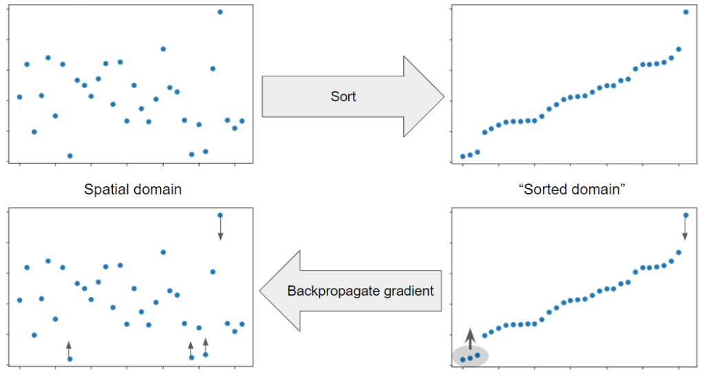
Writing gradient of both of those manually wouldn’t be very hard… But in JAX it is already done for us, we already got both operations implemented as part of the library, and we can JIT the resulting gradient evaluation, so nothing left for us but to design a loss and optimize it!

Fourier domain optimization – whole science fields and prior work

I have to mention here that optimizing frequency spectra, or backpropagating through them is actually very common and it is used all the time in medical imaging, computational imaging, radio / astronomical imaging, and there are types of microscopy and optics based on it. Those are super fascinating fields and it probably takes lifetime to study those properly, and I am complete layman when it comes to those – but before I conclude the section, I’ll link a talk by Katie Bouman on the recent event horizon telescope which also does frequency domain processing (and in a way uses the whole Earth as a such Fourier telescope – no big deal! 🙂 ).

Setting up loss function and optimization tricks

As I mentioned in my previous post, designing a good loss function is the main part of the problem when dealing with optimization-based techniques… (along things like convergence, proofs of optimality, conditioning, and better optimization shemes… but even many “serious” papers don’t really care about those!).

So what would be the loss component of our blue noise function? I came up with the following:

This is just an example – again, I wanted to focus on the technique, not on the specific results or choices! If you some alternative ideas, please let me know in the comments below 👇.

Again, code for this blog post is available and immediately reproducible here.

There are also many “meta” tuning parameters – what would be our low frequency cutoff point? How do we balance each loss component? What histogram shape we want? The best part – you can try and adjust any of those to taste and to your liking and specific use-case. 🙂

When running optimization on such a compound loss function, I almost immediately encountered getting stuck in some “dreaded” local minima. On the other hand, when optimizing only for the loss sub-components, the optimization was converging nicely. Inspired by the stochastic gradient descent that is commonly known to generalize and converge to better global minima than any batch based / whole dataset optimization, I used this observation to “stochasticize” / randomize the loss function slightly (to help “nudge” the solutions out of the local minima or saddle points).

The idea is simple – scale the loss components by a random factor, different per each gradient update / iteration. Given my “complete” loss function comprised of three sub-components, I scale each one by a random uniform in the range 0-1. This seemed to work very well and help optimization to achieve plausibly looking results without local minima.

As a final step, I run fine-tuning on the histogram only part (could as well just force-normalize, but reused existing code), as without it histograms were “almost” perfect. I think in practice it wouldn’t matter, but why not have a “perfect” unbiased dithering pattern if we can?

Results

Without further ado, after playing for a few tries with different loss components and learning rates, I got a following 64×64 dithering matrix:

And the following spectrum:

One of the components of the loss that is hardest to optimize for is spectrum uniformity. It makes sense to me intuitively – smoothness of the spectrum means that we can propagate values only between ajdacent frequencies, which then affect all pixels and most likely cancel each other out (especially together with other loss components). Most likely a smarter metric (maybe just optimize directly for desired value in buckets? 🙂 ) would yield better results – or better optimizer, or simply running the optimization for longer than a few minutes, but they are not too bad at all! And it’s not 100% clear to me if it is necessary to have perfectly uniform spectrum.

Since those blue noise dithering matrices would be used after tiling for dithering, I tested how they look on 2bit dithering of an RGB image from Kodak dataset:

The difference is striking – which is not surprising at all. It’s even more visible on a 1-but quantized image (though here we can argue that both look unacceptably low quality / “retro” heh):

Still – in the blue noise dithered version you can actually read the text and I think it looks much better! I haven’t compared with any other techniques and not sure if it really matters in practice, especially for something so simple as dithering that has also more expensive, better alternatives (like error diffusion).

Conclusions

I have presented an alternative approach to designing dither matrices – by directly optimizing the energy function on the frequency spectrum, and the value range, and running a gradient descent to optimize for those objectives.

I haven’t really exhausted the topic and there are many interesting follow-up questions:

• how a triangular or Gaussian noise value PDF affects the optimization?
• What is the desired frequency cutoff point for dithering?
• How to balance the loss terms and how to express smoothness more elegantly? Does the smoothness matter?
• Would better optimization schemes like e.g. momentum based yield even faster convergence?
• What about extending it to more dimensions? Projection-slice property of Fourier transform acts against us, but maybe we can optimize frequency in 2D, and some other metric in other dimensions?

…and probably many more, that I don’t plan to work more on for now, but I hope my post content and immediately-reproducible Python JAX code that I included will inspire you to some further (and smarter than my brute-force!) experiments.

Post scriptum / digression – optimization vs deep learning – which one is “expensive”?

While writing this post, I contemplated on something quite surprising – a digression on optimization and its relationship with deep learning – something I found counter-intuitive and paradoxically converse views between practitioners and academia: When switching from working in “the industry” on mostly production (and applied research), to working in research groups and interacting with academics, I immediately encountered some opposite views on deep neural networks.

For me, a graphics practitioner, they were cool, higher quality than some previous solutions, but impractical and too slow for most real product applications. At the same time, I have heard from at least some academics that neural networks were super efficient, albeit somewhat sloppy approximations.

What the hell, where does this disconnect come from? Then, reading more about state of the art methods prior to DL revolution, I realized that most of them were using optimization of some energy function on a whole problem and solving a complex, non-linear and huge problem with gradient descent (for example on a non-linear system where every unknown is a pixel of an image!) per every single instance of the problem, and from scratch.

By comparison, artificial neural networks might seem brute-force and wasteful to a practitioner, (per every pixel, hundreds if not thousands/millions of huge matrix multiplies of mostly meaningless weights and “features”, and gigantic waste of memory bandwidth) but the key difference is that the expensive “loss” optimization happens offline. In the runtime/evaluation it is “just” passing data through all the layers and linear algebra 101 arithmetic.

So yeah, our perspectives were very different. 🙂 But I am also sure that if we care about e.g. power consumption, energy efficiency and “operations per pixel”, we can take the idea of optimizing offline much further.