
In previous two parts of this blog post mini-series I described basic uses mentioned blue noise definition, referenced/presented 2 techniques of generating blue noise and one of many general purpose high-frequency low-discrepancy sampling sequences.
In this post, we will look at some more practical example – use of (blue) noise in 2D image dithering for quantization!
You can find Mathematica notebook for this post here and its pdf version here.
Bit quantization in 2D
Finally, we are getting to some practical use case. When you encode your images in 8 bits (typical framebuffer) – you are quantizing. When you encode your GBuffers, render targets and others – you are quantizing. Even typical 8 bit is enough to cause some banding on very smooth, slow gradients – like skies or lens flares.
We will cover here a more extreme example though – extreme 3 bit quantization of a linear gradient.

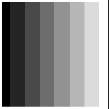
We call those quantization artifacts – 8 visible bands the “banding” effect.
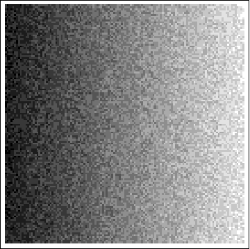
As we learned in previous parts, we can try to fix it by applying some noise. At first, let’s try regular, white noise:
Doesn’t look too good. There are 2 problems:
- “Clumping” of areas, identical to one we have learned before and we will address it in this post.
- Still visible “bands” of unchanged values – around center of bands (where banding effect was not contributing to too much error.
Error visualized.
Those bands are quite distracting. We could try ti fix them by dithering even more (beyond the error):
This solves this one problem! However image is too noisy now.
There is a much better solution that was described very well by Mikkel Gjoel.
Using triangular noise distribution fixes those bands without over-noising the image:
Use of triangular noise distribution.
Since this is a well covered topic and it complicates analysis a bit (different distributions), I will not be using this fix for most of this post. So those bands will stay there, but we will still compare some distributions.
Fixed dithering patterns
In previous part we looked at golden ratio sequence. It is well defined and simple for 1D, however doesn’t work / isn’t defined in 2D (if we want it to be uniquely defined).
One of oldest, well known and used 2D dithering patterns is so called Bayer matrix or ordered Bayer. It is defined as a recursive matrix of a simple pattern for level zero:
1 2
3 0
With next levels defined as:
4*I(n-1) + 1 —– 4*I(n-1) + 2
4*I(n-1) + 3 —– 4*I(n-1) + 0
It can be replicated with a simple Mathematica snippet:
Bayer[x_, y_, level_] :=
Mod[Mod[BitShiftRight[x, level], 2] + 1 + 2*Mod[BitShiftRight[y, level], 2],
4] + If[level == 0, 0, 4*Bayer[x, y, level – 1]]
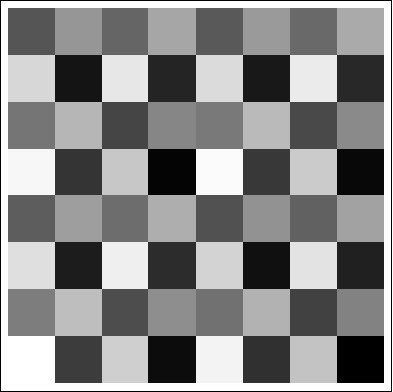
8×8 ordered Bayer matrix
What is interesting (and quite limiting) about Bayer is that due to its recursive nature, signal difference is maximized only in this small 2×2 neighborhood, so larger Bayer matrices add more intermediate steps / values, but don’t contribute much to any visible pattern difference. Therefore most game engines that I have seen used up to 4×4 Bayer pattern with 16 distinctive values.
If you plot a periodogram (frequency spectrum) of it, you will clearly see only 2 single, very high frequency dots!

2D periodogram – low frequencies are in the middle and high frequencies to the sides.
Obviously signal has some other frequencies, but much lower intensities… Plotting it in log scale fixes it:
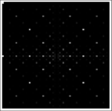
So on one hand, Bayer matrix has lots of high frequency – would seem perfect for dithering. However presence of strong single frequency bands tends to alias it heavily and produce ugly pattern look.
This is our quantized function:
If you have been long enough playing with computers to remember 8 bit or 16 bit color modes and palletized images, this will look very familiar – as lots of algorithms used this matrix. It is very cheap to apply (a single look up from an array or even bit-magic ops few ALU instructions) and has optimum high frequency content. At the same time, it produces this very visible unpleasant patterns. They are much worse for sampling and in temporal domain (next 2 parts of this series), but for now let’s have a look at some better sequence.
Interleaved gradient noise
The next sequence that I this is working extremely well for many dithering-like tasks, is “interleaved gradient noise” by Jorge Jimenez.
Formula is extremely simple!
InterleavedGradientNoise[x_, y_] :=
FractionalPart[52.9829189*FractionalPart[0.06711056*x + 0.00583715*y]]
But the results look great, contain lots of high frequency and produce pleasant, interleaved smooth gradients (be sure to check Jorge’s original presentation and his decomposition of “gradients”):

What is even more impressive is that such pleasant visual pattern was invented by him as a result of optimization of some “common web knowledge” hacky noise hashing functions!
Unsurprisingly, this pattern has periodogram containing frequencies that correspond to those interleaved gradients + their frequency aliasing (result of frac – similar to frequency aliasing of a saw wave):
And the 3D plot (spikes corresponding to those frequency):
Just like with Bayer, those frequencies will be prone to aliasing and “resonating” with frequencies in source image, but almost zero low frequencies given nice, clean smooth look:
Some “hatching” patterns are visible, but they are much more gradient-like (like the name of the function) and therefore less distracting.
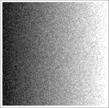
Blue noise
Finally, we get again to using a blue noise pre-generated pattern. To recall from previous part, blue noise is loosely defined as a noise function with small low frequency component and uniform coverage of different frequencies. I will use here a pattern that again I generated using my naive implementation of “Blue-noise Dithered Sampling” by Iliyan Georgiev and Marcos Fajardo.
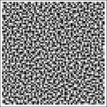
So I generated a simple 64×64 wrapping blue noise-like sequence (a couple hours on an old MacBook):
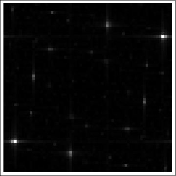
It has following periodogram / frequency content:

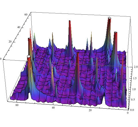
And in 3D (who doesn’t love visualizations?! 😀 ):
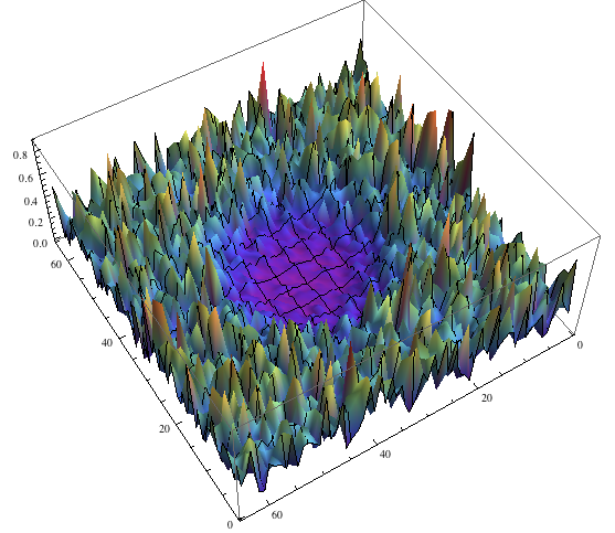
Compared to white noise, it has a big “hole” in the middle, corresponding to low frequencies.
White noise vs blue noise in 2D
At the same time, it doesn’t have linear frequency increase for higher frequencies, like audio / academic definition of blue noise. I am not sure if it’s because my implementation optimization (only 7×7 neighborhood is analyzed + not enough iterations) or the original paper, but doesn’t seem to impact the results for our use case in a negative way.
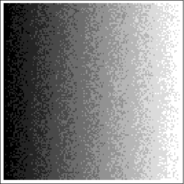
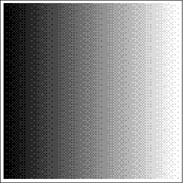
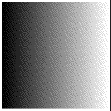
Without further ado, results of dithering using 2D blue noise:
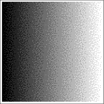
It is 64×64 pattern, but it is optimized for wrapping around – so border pixels error metric is computed with taking into account pixels on the other side of the pattern. In this gradient, it is repeated 2×2.
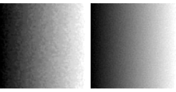
And this is how it compared to regular white noise:
White noise vs blue noise
Because of high frequency contents only, you can’t see this problematic “clumping” effect.
It also means that if we oversample (like with all those new fancy 1080p -> 1440p -> 2160p displays), blur it or apply temporal (one of next parts), it will be more similar to original pattern! So when we filter them with 2-wide Gaussian:
Left: Gaussian-filtered white noise dithering. Right: Gaussian-filtered blue noise dithering.
And while I said we will not be looking at triangle noise distribution in this post for simplicity, I couldn’t resist the temptation of comparing them:
White noise vs blue noise with triangular distribution remapping applied.
I hope that this at least hints at an observation that with a good, well distributed large enough blue noise fixed pattern you might get results maybe not the same quality level of error diffusion dithering, but in that direction and orders of magnitude better than standard white noise.
All four compared
Just some visual comparison of all four techniques:

White noise, blue noise, Bayer, interleaved gradient noise

And with the triangular remapping:

My personal final recommendations and conclusions and here would be:
- Whenever possible, avoid ordered Bayer! Many game engines and codebases still use it, but it produces very visible unpleasant patterns. I still see it in some currently shipped games!
- If you cannot spare any memory look-ups but have some ALU, use excellent interleaved gradient noise by Jorge Jimenez. It produces much more pleasant patterns and is extremely cheap with GPU instruction set! However patterns are still noticeable and it can alias.
- Blue noise is really great noise distribution for many dithering tasks and if you have time to generate it and memory to store it + bandwidth to fetch, it is the way to go.
- White noise is useful for comparison / ground truth. With pixel index hashing it’s easy to generate, so it’s useful to keep it around.
Summary
In this part of the series, I looked at the topic of quantization of 2D images for the purpose of storing them at limited bit depth. I analyzed looks and effects of white noise, ordered Bayer pattern matrices, interleaved gradient noise and blue noise.
In next part of the series (coming soon), we will have a look at the topic of dithering in more complicated (but also very common) scenario – uniform sampling. It is slightly different, because often requirements are different. For example if you consider rotations, values of 0 and 2pi will “wrap” and be identical – therefore we should adjust our noise distribution generation error metric for this purpose. Also, for most sampling topics we will need to consider more that 1 value of noise.
Edit 10/31/2016: Fixed triangular noise remapping to work in -1 – 1 range instead of -0.5-1.5. Special thanks to Romain Guy and Mikkel Gjoel for pointing out the error.
References
http://loopit.dk/banding_in_games.pdf “Banding in games”, Mikkel Gjoel
https://engineering.purdue.edu/~bouman/ece637/notes/pdf/Halftoning.pdf C. A. Bouman: Digital Image Processing – January 12, 2015
B. E. Bayer, “An optimum method for two-level rendition of continuous-tone pictures”, IEEE Int. Conf. Commun., Vol. 1, pp. 26-1 1-26-15 (1973).
http://www.iryoku.com/next-generation-post-processing-in-call-of-duty-advanced-warfare “Next generation post-processing in Call of Duty: Advanced Warfare”, Jorge Jimenez, Siggraph 2014 “Advances in Real Time Rendering in games”
“Blue-noise Dithered Sampling”, Iliyan Georgiev and Marcos Fajardo
https://github.com/bartwronski/BlueNoiseGenerator
http://www.reedbeta.com/blog/quick-and-easy-gpu-random-numbers-in-d3d11/ “Quick And Easy GPU Random Numbers In D3D11”, Nathan Reed

Pingback: Dithering in games – mini series | Bart Wronski
Pingback: Small float formats – R11G11B10F precision | Bart Wronski
Pingback: Animating Noise For Integration Over Time « The blog at the bottom of the sea
Pingback: Dithering part two – golden ratio sequence, blue noise and highpass-and-remap | Bart Wronski
Pingback: The Unreasonable Effectiveness of Quasirandom Sequences | Extreme Learning
Pingback: “Optimizing” blue noise dithering – backpropagation through Fourier transform and sorting | Bart Wronski
This overnoising with triangular remapping looks great, but only until you use it on near-black or near-white parts of the image. In this case blacks become slightly lighter (about 20% of the quantization step), and the whites become a bit darker. This happens because the noise becomes large enough in amplitude to overshoot over half a quantization step. This normally cancels out on average, but on the borders it’s not, due to clipping. The problem can be overcome by tuning the initial color value beyond black/white, and only then applying the noise, so that the expected value of the result is equal to the input color.
I’ve been pulling my hair out after trying to use interleaved gradient noise as a 2D seed per pixel. The common solution is to just generate two uncorrelated noise patterns, but IGN is inherently correlated. Is there some obvious workaround I am missing?
You can try different seeds and moving patterns around – even offline, brute-force search through different offsets and compute correlations, picking the one that is closest to zero. I don’t know if it would work, but might give it a try!
An alternative is to compute (noise + golden number) % 1 to get the second one, but this one works rather poor in my experience.