The goal of this post is to show how to download our own data stored and used by internet services to generate personalized stats / charts like below and will show step-by-step how to do it using colab, Python, pandas, and matplotlib.

Disclaimer: I wrote this post as a private person, not representing my employer in any way – and from a 100% outside perspective.

Intro / motivation

When we decide to use one particular internet service over the other, it is based on many factors and compromises – we might love our choices, but still find ourselves missing certain features.

Seeing “year in review” from Spotify shared by friends made me envious. Google Play Music that I personally use doesn’t have such a cool feature and didn’t give me an opportunity to ponder and reflect on the music I listened to in the past year (music is a very important part of my life).

Luckily, the internet is changing and users, governments, as well as internet giants are becoming more and more aware of what it means for a user to “own their data”, request it, and there is a need for increased transparency (and control/agency over data we generate while using those servies). Thanks to those changes (materializing themselves in improved company terms of service, and regulatory acts like GDPR or California Consumer Privacy Act), on most websites and services we can request or simply download the data that those collect to operate.

Google offers such a possibility in a very convenient form (just a few clicks) and I used my own music playing activity data together with Python, pyplot, and pandas to create a personalized “year in review” chart(s) and given how cool and powerful, yet easy it is, decided to share it in a short blog post.

This blog post comes with code in form of a colab and you should be able to directly analyze your own data there, but more importantly I hope it will inspire you to check out what kind of other user data your might have a creative use for!

Downloading the data

The first step is trivial – just visit takeout.google.com.

Gotcha no 1: Amount of different Google services is impressive (if not a bit overwhelming) and it took me a while to realize that the data I am looking for is not under “Google Play Music“, but under “My Activity”. Therefore I suggest to “Deselect all”, and then select “My Activity”. Under it, click on “All activity data included” and filter to just Google Play Music “My Activity” content:

The nextstep here would be to change the data format from HTML to just JSON – which is super easy to load and parse with any data analysis frameworks or environments.

Finally, proceed to download your data as “one-time archive” and a format that works well for you (I picked a zip archive).

I got a “scary” message that it can take up to a few days to get a download link to this archive, but then got it in less than a minute. YMMV, I suspect that it depends on how much data you are requesting at given time.

Downloaded data

Inside the downloaded archive, my data was in the following file:

Takeout\My Activity\Google Play Music\MyActivity.json

Having a quick look at this JSON file, looks like it contains all I need! For every activity/interaction with GPM, there is an entry with title of the activity (e.g. listened to, searched for), description (which is in fact artist name), time, as well as some metadata:

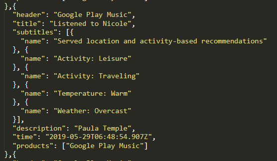
One thing that is interesting is that “subtitles” contain information about “activity” that GPM associated with given time, temperature, and weather outside. This kind of data was introduced between 2019-03-21 (is not included my entries on that date or before) and 2019-03-23 (the first entry with such information). The activity isn’t super accurate, most of them are “Leisure” for me, often even when I was at work or commuting, but some are quite interesting, e.g. it often got “Shopping” right. Anyway, it’s more of a curiosity and I haven’t found great use for it myself, but maybe you will. 🙂

Gotcha no 2: all times described there seem to be in GMT – at least for me. Therefore if you listen to music in any different timezone, you will have to convert it. I simplified my analysis to use pacific time. This results in some incorrect data – e.g. I spent a month this year in Europe and music that I listened to during that time will be marked incorrectly as during some “weird hours”.

Analyzing the data

Ok, finally it’s time for something more interesting – doing data analysis on the downloaded data. I am going to use Google Colaboratory, but feel free to use local Jupyter notebooks or even commandline Python.

Code I used is available here.

Note: this is the first time I used pandas, so probably some pandas experts and data scientists will cringe at my code, but hey, it gets the job done. 🙂

The first step to analyze a local file with a colab is to upload it to the runtime using the tab on the left of the colab window – see the screenshot below. I have uploaded just the MyActivity.json without any of the folder structure. If you use local scripts, this step is unnecessary. as you can specify full local path

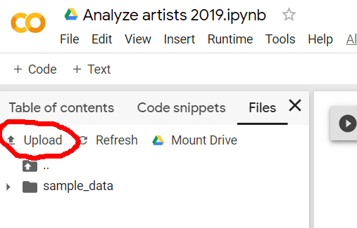
Gotcha no 3: Note that uploading files doesn’t associate them with your notebook, account used to open colab or anything like that – just with current session in the current runtime, so anytime you restart your session, you will have to reupload the file(s).

Time to code! We will start with loading some Python libraries and set the style of plots to a bit prettier:

import pandas as pd
import numpy as np
import seaborn as sns
import matplotlib.pyplot as plt
plt.style.use('seaborn-whitegrid')

Then we can read the JSON file as Pandas dataframe – I think of it as of table in SQL, which is probably oversimplification, but worked for my simple use-case. This step worked for me right away and required no data preprocessing:

df = pd.read_json('MyActivity.json')
print(df.columns)

Index(['header', 'title', 'subtitles', 'description', 'time', 'products',
       'titleUrl'],
      dtype='object')
                         title description                      time
0  Listened to Jynweythek Ylow  Aphex Twin  2019-12-31T23:33:55.865Z
1       Listened to Untitled 3  Aphex Twin  2019-12-31T23:26:23.465Z
2                Listened to 4  Aphex Twin  2019-12-31T23:22:46.829Z
3               Listened to #3  Aphex Twin  2019-12-31T23:15:02.427Z
4           Listened to Nanou2  Aphex Twin  2019-12-31T23:11:36.944Z
5  Listened to Alberto Balsalm  Aphex Twin  2019-12-31T23:06:25.999Z
6             Listened to Xtal  Aphex Twin  2019-12-31T23:01:32.538Z
7       Listened to Avril 14th  Aphex Twin  2019-12-31T22:59:27.321Z
8        Listened to Fingerbib  Aphex Twin  2019-12-31T22:55:37.856Z
9              Listened to #17  Aphex Twin  2019-12-31T22:53:32.866Z

This is great! Now a bit of clean up. We want to apply the following:

• For easier further coding, rename the unhelpful “description” to “artist”,
• Convert the string containing date and time to pandas datetime for easier operations and filtering,
• Convert the timezone to the one you want to use as a reference – I used single one (US Pacific Time), but nothing prevents you from using different ones per different entries, e.g. based on your locations if you happen to have them e.g. extracted from other internet services,
• Filter only “Listened to x/y/z” activities, as I interested in analyzing what I was listening to, and not e.g. searching for.

df.rename(columns = {'description':'artist'}, inplace=True)
df['time'] = df['time'].apply(pd.to_datetime)
df['time'] = df['time'].dt.tz_convert('America/Los_Angeles')
listened_activities = df.loc[df['title'].str.startswith('Listened to')]

Now we have a dataframe containing information about all of our listening history. We can do quite a lot with it, but I didn’t care for specific “tracks” (analyzing this could be useful to someone), so instead I went to a) filter only activities that happened in 2019, and b) group all events of listening to a single artist.

For the step b), let’s start with just annual totals. We group all activities and use size of each group as a new column (total play count).

listened_activities_2019 = listened_activities.loc[(listened_activities['time'] >= '2019-01-01') & (listened_activities['time'] < '2020-01-01')]
artist_totals = listened_activities_2019.groupby('Artist').size().reset_index(name='Play counts')
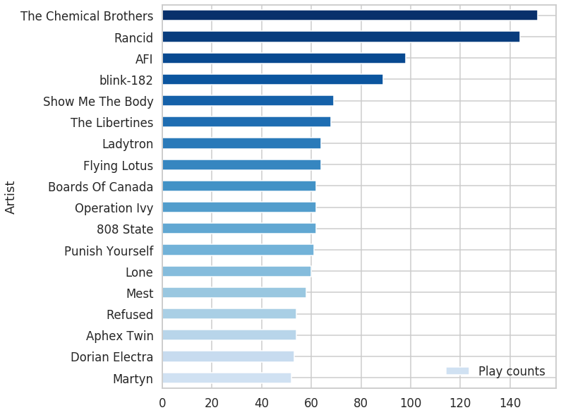
top = artist_totals.sort_values('Play counts', ascending=False).set_index('Artist')[0:18]
print(top)

                       Play counts
Artist                            
The Chemical Brothers          151
Rancid                         144
AFI                             98
blink-182                       89
Show Me The Body                69
The Libertines                  68
Ladytron                        64
Flying Lotus                    64
Boards Of Canada                62
Operation Ivy                   62
808 State                       62
Punish Yourself                 61
Lone                            60
Mest                            58
Refused                         54
Aphex Twin                      54
Dorian Electra                  53
Martyn                          52

This is exactly what I needed. It might not be surprising (maybe a little bit, I expected to see some other artists there – but they were soon after – I am a “long tail” type of listener), but cool and useful nevertheless.

Now let’s plot it with matplotlib. I am not pasting all the code here as there is a bit of boilerplate to make plots pretties, so feel free to check the colab directly. Here is the resulting plot:

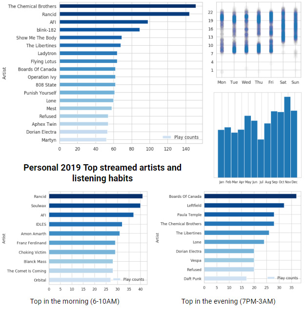
From this starting point, let your own creativity and imagination be your guide. Some ideas that I tried and had fun with:

• hourly or weekly listening activity histograms,
• monthly listening totals / histograms,
• checking whether I tend to listen to different music in the evening versus the morning (I do! Very different genres to wake up vs unwind 🙂 ),
• weekly time distributions.

All of those operations are very simple and mostly intuitive in Python + pandas – you can extract things like hour, day of the week, month etc. directly from the datetime column and then use simple combinations of conditional statements and/or groupings.

Some of those queries/ideas that I ran for my data are aggregated in a single plot below:

Summary

Downloading and analyzing my own data for Google Play Music was really easy and super fun. 🙂

I have to praise here all of the following:

• User friendly and simple Google data / activity downloading process, and its data produced in a very readable/parseable format,
• Google Colab being an immediate, interactive environment that makes it very easy to run code on any platform and share it easily,
• Pandas as data analysis framework – I was skeptical and initially would have preferred something SQL-like, but it was really easy to learn for such a basic use case (with help of the documentation and Stackoverflow 🙂 ),
• As always, how powerful numpy and matplotlib (despite its quite ugly looking defaults and tricks required to do simple things like centering entries on label “ticks”) are – but those are already kind of industry standards, so won’t add here more compliments.

I hope this blog post inspired you to download and tinker with your own activity data. Hopefully this will be not just fun, but also informative to understand what is stored – and you can even judge what do you think is really needed for those services to run well. The activity data I downloaded from Google Play Music looks like a reasonable, bare minimum that is useful to drive the recommendations.

To conclude, I think that anyone with even the most basic coding skills can have tons of fun analyzing their own activity data – combining information to create personally meaningful stats, exploring own trends and habits, extending functionalities, or adding (though only for yourself and offline) completely new features for commercial services written by large teams.