
Gaussian filters are the bread and butter of signal and image filtering. They are isotropic and radially symmetric, filter out high frequencies extremely well, and just look pleasant and smooth.
In this post I will cover two of my favorite small Gaussian (and Gaussian-like) filtering “tricks” and caveats that are not appreciated by textbooks, but are important in practice.
The first one is binomial filters – a generalization of literally the most useful (in my opinion) filter in computer graphics, image processing, and signal processing.
The second one is discretizing small sigma Gaussians – did you ever try to compute a Gaussian of sigma 0.3 and wonder why you get close to just [0.0, 1.0, 0.0]?
You can treat this post as two micro-posts that I didn’t feel like splitting and cluttering too much.
Binomial filter – fast and great approximation to Gaussians
First up in the bag of simple tricks is “binomial filter”, as called by Aubury and Tuk.
This one is in an interesting gray zone – if you do any signal or image filtering on CPUs or DSPs, it’s almost certain you used them (even if you didn’t know under such a name). On the other hand, through almost ~10 years of GPU programming I have not heard of them.
The reason is their design is perfect for fixed point arithmetic (but I’d argue that is actually also neat and useful with floats).
Simplest example – [1, 2, 1] filter
Before describing what “binomial” filters are, let’s have a look at the simplest example of them – a “1 2 1” filter.
[1, 2, 1] refers to multiplier coefficients that then are normalized by dividing by 4 (a power of two -> can be implemented either by a simple bit shift, or super efficiently in hardware!).
In a shader you can use directly a [0.25, 0.5, 0.25] form instead – and for example on AMD hardware those small inverse power of two multipliers can become just instruction modifiers!
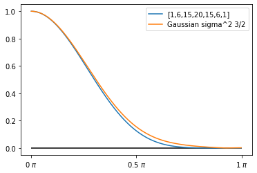
This filter is pretty close to a Gaussian filter with a sigma of ~0.85.
Here is the frequency response of both:

For the Gaussian, I used a 5 point Gaussian to prevent excessive truncation -> effective coefficients of [0.029, 0.235, 0.471, 0.235, 0.029].
So while the binomial filter here deviates a bit from the Gaussian in shape, but unlike this sigma of Gaussian, it has a very nice property of reaching a perfect 0.0 at Nyquist. This makes this filter a perfect one for bilinear upsampling.
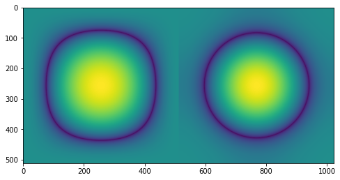
In practice, this truncation and difference is not going to be visible for most signals / images, here is an example (applied “separably”):

Last panel is the difference enhanced x10. It is the largest on a diagonal line due to how only a “true” Gaussian is isotropic. (“You say Gaussians have failed us in the past, but they were not the real Gaussians!” 😉 )
For quick visualization, here is the frequency response of both with a smooth isoline around 0.2:
As you can see, Gaussian is perfectly radial and isotropic, while a binomial filter has more “rectangular” response, filtering less of the diagonals.
Still, I highly recommend this filter anytime you want to do some smoothing – a) extremely fast to implement, simple to memorize, b) just 3 taps in a single direction, so can be easily done also as non-separable 9-tap one c) has a zero at Nyquist, making it great for both downsampling, as well as upsampling (removed grid artifacts!).
Binomial filter coefficients
This was the simplest example of the binomial filter, but what does it have to do with the binomial coefficients or distribution? It is the third row from Pascal’s triangle.
You can construct the next Binomial filter by taking the next row from it.
Since we typically want odd-sized filters, I would compute the following row (ok, I have a few of them memorized) of “n over from 0 to 4”:
[1, 4, 6, 4, 1]
The really cool thing about Pascal’s triangle rows is that they always sum to a power of two – this means that here we can normalize simply by dividing by 16!
…or alternatively you can completely ignore the “binomial” part, and look at it like a repeated convolution. If we keep repeating convolving [1, 1] with itself, we get next binomial coefficients:
a = np.array([1, 1])
b = np.array([1])
for _ in range(7):
  print(b, np.sum(b))
  b = np.convolve(a, b)

[1] 1
[1 1] 2
[1 2 1] 4
[1 3 3 1] 8
[1 4 6 4 1] 16
[ 1  5 10 10  5  1] 32
[ 1  6 15 20 15  6  1] 64
At the same time, looking at coefficients of (a + b) ^ n == (a + b)(a + b)…(a + b) and is exactly the same as repeated convolution.
From this repeated convolution we can also see why the coefficients sum is powers of two – we always get 2x more from convolving with [1, 1].
Larger binomial filters
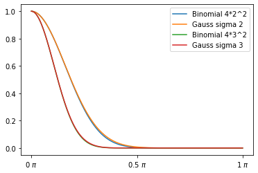
Here the [1, 4, 6, 4, 1] is approximately equivalent to a Gaussian of sigma ~1.03.

The difference starts to become really tiny. Similarly, the next two binomial filters:

Wider and wider binomial filters
Now something that you might have noticed on the previous plot is that I have marked Gaussian sigma squared as 3 and 4. For the next ones, the pattern will continue, and distributions will be closer and closer to Gaussian. Why is that so? I like how the Pascal triangle relates to a Galton board and binomial probability distribution. Intuitively – the more independent “choices” a falling ball can make, the closer final position distribution will resemble the normal one (Central Limit Theorem). Similarly by repeating convolution with a [1, 1] “box filter”, we also get closer to a normal distribution. If you need some more formal proof, wikipedia has you covered.
Again, all of them will sum up to a power of two, making a fixed point implementation very efficient (just widening multiply adds, followed by optional rounding add and a bit shift).
This leads us to a simple formula. If you want a Gaussian with a certain sigma, square it, and compute a binomial of 4*sigma^2 over x.
For example for sigma 2 and 3, almost perfect match:
Binomial filter use – summary
That’s it for this trick!
Admittedly, I rarely had uses for anything above [1, 4, 6, 4, 1], but I think it’s a very useful tool (especially for image processing on a CPU / DSP) and worth knowing the properties of those [1, 2, 1] filters that appear everywhere!
Discretizing small sigma Gaussians
Gaussian (normal) distribution probability distribution is well defined on an infinite, continuous domain – but it never reaches zero. When we want to discretize it for filtering a signal or an image – things become less well defined.
First of all, the fact that it never reaches zero means that we should use “infinite” filters… Luckily, in practice it decays so quickly that using ceil(2-3 sigma) for radius is enough and we don’t need to worry about this part of the discretization.
Another one is more troublesome and ignored by most textbooks or articles on Gaussian – that we point sample a probability density function, which can work fine for any larger filters (sigma above ~0.7), but definitely cause errors and undersampling for small sigmas!
Let’s have a look at an example and what’s going on there.
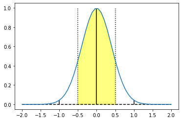
Gaussian sigma of 0.4…?
If we have a look at Gauss of sigma 0.4 and try to sample the (unnormalized) Gaussian PDF, we end up with:

The values sampled at [-1, 0, 1] end up being: [0.0438, 0.9974, 0.0438].
This is… extremely close to 0.0 for the non-center taps.
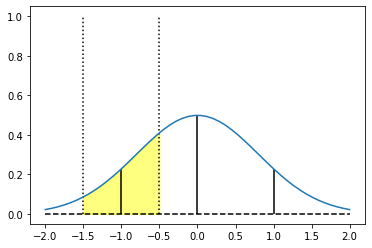
At the same time, if you look at all the values at the pixel extent, it doesn’t seem to correspond well to the sampled value:
If you wonder if we should look at the pixel extent and treat it as a little line/square (oh no! Didn’t I read the memo..?), the answer is (as always…) – it depends. It assumes that nearest-neighbor / box would be used as the reconstruction function of the pixel grid. Which is not a bad assumption with contemporary displays actually displaying pixels, and it simplifies a lot of the following math.
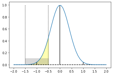
On the other hand, value for the center is clearly overestimated under those assumptions:
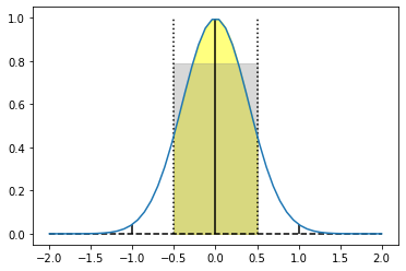
I want to emphasize here – this problem is +/- unique to small Gaussians. If we look only at mere sigma of 0.8, middle-side samples start to look much closer to proper representative value:
Yes, edges and the center still don’t match, but with increasing radii, this problem becomes minimal even there.
Literature that observes this issue (most don’t!) suggests to ignore it; and they are right – but only assuming that you don’t want to use a sigma of anything below 1.0.
Which sometimes you actually want to use; especially when modelling some physical effects. Modeling small Gaussians is also extremely useful for creating synthetic training data for neural networks, or tasks like deblurring.
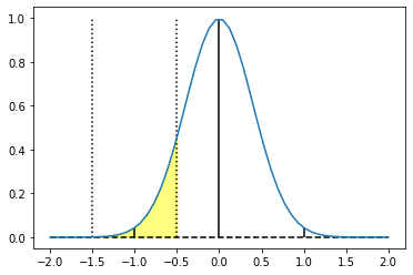
Integrating a Gaussian
So how do we compute an average value of Gaussian in a range?
There is good news and bad news. 🙂
Good news are – this is very well studied, we just need to integrate a Gaussian and we can just use the error function. The bad news… it doesn’t have any nice and closed formula; even in numpy/scipy environment it is treated as a “special” function. (In practice those are often computed by a set of approximations / tables followed by Newton-Raphson or similar corrections to get to desired precision.)
We just evaluate this integral at pixel extent endpoints, and subtract them and divide it by two.
The formula for a Gaussian integral “corrected” this way becomes:
def gauss_small_sigma(x: np.ndarray, sigma: float):
  p1 = scipy.special.erf((x-0.5)/sigma*np.sqrt(0.5))
  p2 = scipy.special.erf((x+0.5)/sigma*np.sqrt(0.5))
  return (p2-p1)/2.0
Is it a big difference? For small sigmas, definitely! For the sigma of 0.4, it becomes [0.1056, 0.7888, 0.1056] instead of [0.0404, 0.9192, 0.0404]!
We can see how good is this value representing the average on the plots:
When we renormalize the coefficients, we get this huge difference.
The difference is also (hopefully) visible with the naked eye:

Verifying the model and some precomputed values
To verify the model, I also plotted a continuous Gaussian frequency response (which is super usefully also a Gaussian, but with an inverse sigma!) and compared it to two small sigma filters, 0.4 and 0.6:
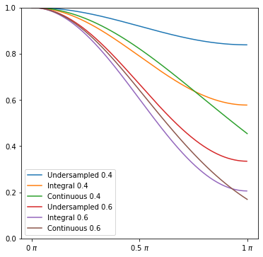
The difference is dramatic for the sigma of 0.4, and much smaller (but definitely still visible; underestimating “real” sigma) for 0.6.
How does it fare in 2D? Luckily, with error function, we can still use a product of two error functions (separability!). However, I expected that it won’t be radially symmetric and fully isotropic anymore (we are integrating its response with rectangles), but luckily, it’s actually not bad and way better than undersampled Gaussian:

Plot shows that the integrated Gaussian has very nicely radially symmetric frequency response until we start getting close to Nyquist and very high frequencies (which is expected) – looks reasonable to me, unlike the undersampled Gaussian which suffers from both this problem, diamond-like response in lower frequencies, and being overall far away in the response shape/magnitude from the continuous one.
Finally, I have tabulated some small sigma Gaussian values (for quickly plugging those in if you don’t have time to compute). Here’s a quick cheat sheet:
| Sigma | Undersampled | Integral | Mean relative error |
|---|---|---|---|
| 0.2 | [0., 1., 0.] | [0.0062, 0.9876, 0.0062] | 67% |
| 0.3 | [0.0038, 0.9923, 0.0038] | [0.0478, 0.9044, 0.0478] | 65% |
| 0.4 | [0.0404, 0.9192, 0.0404] | [0.1056, 0.7888, 0.1056] | 47% |
| 0.5 | [0.1065, 0.787, 0.1065] | [0.1577, 0.6845, 0.1577] | 27% |
| 0.6 | [0.1664, 0.6672, 0.1664] | [0.1986, 0.6028, 0.1986] | 14% |
| 0.7 | [0.2095, 0.5811, 0.2095] | [0.2288, 0.5424, 0.2288] | 8% |
| 0.8 | [0.239, 0.522, 0.239] | [0.2508, 0.4983, 0.2508] | 5% |
| 0.9 | [0.2595, 0.481, 0.2595] | [0.267, 0.466, 0.267] | 3% |
| 1.0 | [0.2741, 0.4519, 0.2741] | [0.279, 0.442, 0.279] | 2% |
To conclude this part, my recommendation is to always consider the integral if you want to use any sigmas below 0.7.
And for a further exercise for the reader, you can think of how this would change under some different reconstruction function (hint: it becomes a weighted integral, or an integral of convolution; for the box / nearest neighbor, the convolution is with a rectangular function).

Pingback: Study of smoothing filters – Savitzky-Golay filters | Bart Wronski
Pingback: Removing blur from images – deconvolution and using optimized simple filters | Bart Wronski
Pingback: Progressive image stippling and greedy blue noise importance sampling | Bart Wronski
Pingback: Gradient-descent optimized recursive filters for deconvolution / deblurring | Bart Wronski