Dithering part one – simple quantization

Introduction

First part of this mini-series will focus on more theoretical side of dithering -some history and applying it for 1D signals and to quantization. I will try to do some frequency analysis of errors of quantization and how dithering helps them. It is mostly theoretical, so if you are interested in more practical applications, be sure to check the index and other parts.

You can find Mathematica notebook to reproduce results here and the pdf version here.

What is dithering?

Dithering can be defined as intentional / deliberate adding of some noise to signal to prevent large-scale / low resolution errors that come from quantization or undersampling.

If you have ever worked with either:

Audio signals,
90s palletized image file formats.

You must have for sure encountered dithering options that by adding some noise and small-resolution artifacts “magically” improved quality of audio files or saved images.

However, I found on Wikipedia quite an amazing fact about when dithering was first defined and used:

…[O]ne of the earliest [applications] of dither came in World War II. Airplane bombers used mechanical computers to perform navigation and bomb trajectory calculations. Curiously, these computers (boxes filled with hundreds of gears and cogs) performed more accurately when flying on board the aircraft, and less well on ground. Engineers realized that the vibration from the aircraft reduced the error from sticky moving parts. Instead of moving in short jerks, they moved more continuously. Small vibrating motors were built into the computers, and their vibration was called dither from the Middle English verb “didderen,” meaning “to tremble.” Today, when you tap a mechanical meter to increase its accuracy, you are applying dither, and modern dictionaries define dither as a highly nervous, confused, or agitated state. In minute quantities, dither successfully makes a digitization system a little more analog in the good sense of the word.

— Ken Pohlmann, Principles of Digital Audio

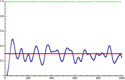
This is inspiring and interesting historical fact and as I understand it that it works by avoiding bias in computations and resonances by randomly breaking up some mechanical vibration feedback loops.

But history aside, let’s look at the dithering process for 1D signals first, like audio.

Dithering quantization of a constant signal

We will start first with analyzing the most boring possible signal – a constant signal. If you know a bit about audio and audio-related DSP, you might ask – but you promised looking at audio and and audio by definition cannot have a constant term! (furthermore, both audio software and hardware deliberately remove so called DC offset)

That’s true and we will have a look at more complicated functions in a second, but first things first.

Imagine that we are doing a 1 bit quantization of a normalized floating point signal. This means we will be dealing with final binary values, 0 or 1.

If our signal is 0.3, simple rounding without any dithering will be the most boring function ever – just zero!

Error is also constant, 0.3 and therefore average is also 0.3. This means that we introduced quite big bias to our signal and completely lost original signal information.

We can try to dither this signal and have a look at results.

Dithering in this case (used rounding function) is applying just plain, random white noise (random value per every element, producing uniform noise spectrum) and adding random value from range (-0.5, 0.5) to the signal prior to quantization.

quantizedDitheredSignal =
Round[constantSignalValue + RandomReal[] – 0.5] & /@ Range[sampleCount];

It’s difficult to see anything here, just that now result of quantization is some random ones and zeros… With (as hopefully expected) more zeros. It’s not terribly interesting signal on its own, but what is quite interesting is the plot of the error and average error.

Ok, we can see that as expected, error is also alternating… but what is quite scary is that error got sometimes bigger (0.7 absolute value)! So our maximum error is worse, pretty unfortunate… however, average noise is:

Mean[ditheredSignalError]
0.013

Much much smaller than original error of 0.3. With sufficiently large amount of samples this error would go towards zero (limit). So error for constant term got much smaller, but let’s have a look at frequency plot of all errors.

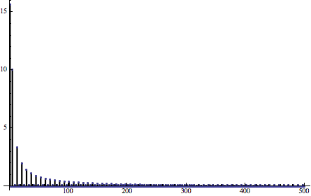
Red plot/spike = frequency spectrum of error when not using dithering (constant, no frequencies). Black – with white noise dithering.

Things are getting more interesting! This shows first major takeaway of this post – dithering distributes quantization error / bias among many frequencies.

We will have a look in the next section how it helps us.

Frequency sensitivity and low-pass filtering

So far we observed that dithering a quantized constant signal:

Increased maximal error.
Almost zeroed average, mean error.
Added constant white noise (full spectral coverage) to the error frequency spectrum, reducing the low-frequency error.

By itself it doesn’t help us too much… However, we are not looking at quantization of any arbitrary mathematical function / signal. We are looking here at signals that will be perceived by humans. Human perception is obviously limited, some examples:

Our vision has a limit of acuity. Lots of people are short-sighted and see blurred image of faraway objects without correction glasses.
We perceive medium scale of detail much better than very high or very low frequencies (small details of very smooth gradients may be not noticed).
Our hearing works in specific frequency range (20Hz -20kHz, but it gets worse with age) and we are most sensitive to middle ranges – 2kHz-5kHz.

Therefore, any error in frequencies closer to upper range of perceived frequency will be much less visible.

Furthermore, our media devices are getting better and better and provide lots of oversampling. In TVs and monitors we have “retina”-style and 4K displays (where it’s impossible to see single pixels), in audio we use at least 44kHz sampling file formats even for cheap speakers that often can’t reproduce more than 5-10kHz.

This means, that we can approximate perceptual look of a signal by low-pass filtering it. Here I did a low pass filtering (padding with zeros on the left -> “ramp up”):

Red – desired non-quantized signal. Green – quantized and dithered signal. Blue – low pass filter of that signal.

Signal starts to look much closer to original, unquantized function!

Unfortunately we started to see some low frequencies that are very visible and were not present in the original signal. We will look at fixing it by using blue noise in part 3 of the series, but for now this is how it could look like with some quasi-noise function that has much less lower frequency content:

This is possible because our quasi-random sequence has following frequency spectrum:

But for now enough looking at simplistic, constant function. Let’s have a look at a sine wave (and if you know Fourier theorem – a building block of any periodic signal!).

Quantizing a sine wave

If we quantize a sine wave with 1 bit quantization, we get a simple… square wave.

Square wave is quite interesting, as it comprises base frequency as well as odd harmonics.

It is interesting property that is used heavily in analog subtractive synthesizers to get hollow/brassy sounding instruments. Subtractive synthesis starts with a complex, harmonically rich sound and filters it by removing some frequencies (with filter parameters varying over time) to shape sounds in desired way.

Square wave frequency spectrum:

But in this post we are more interested in quantization errors! Let’s plot the error as well as frequency spectrum of the error:

In this case we are in much better situation – average error is close to zero! Unfortunately, we still have lots of undesired low frequencies, very close to our base frequency (odd multiplies with decreasing magnitudes). This is known as aliasing or dithering noise – frequencies that were not present in the original signal appear and they have pretty large magnitudes.

Even low-pass filtering cannot help this signal much… As error has so many low frequencies:

Low-pass filtered quantized sine

Low-pass filtered quantized sine error

Let’s have a look at how this changes with dithering. At first sight things don’t improve a lot:

However if we display it as an image, it starts to look better:

And notice how again, quantization error gets distributed among different frequencies:

This looks very promising! Especially considering that we can try to filter it now:

That’s slightly crooked sine, but looks much closer to original one than the non-dithered one with the exception of a phase shift introduced by asymmetrical filter (I am not going to describe or cover it here; it is fixable simply by applying symmetrical filters):

Red – original sine. Green – low pass filtered undithered signal. Blue – low pass filtered dithered signal.

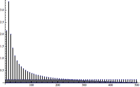
Plotting both error functions confirms numerically that error is much smaller:

Red – error of low-pass filtered non-dithered signal. Blue – error of low-pass filterer dithered signal.

Finally, let’s just quickly look at a signal with better dithering function containing primarily high frequencies:

Upper image – white noise function. Lower image – a function containing more higher frequencies.

Low-pass filtered version dithered with a better function – almost perfect results if we don’t count filter phase shift!

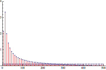
And finally – all 3 comparisons of error spectra:

spectrum_quantization_noise_golden__comparison_sine.gif

Red – undithered quantized error spectrum. Black – white noise dithered quantized error spectrum. Blue – noise with higher frequencies ditherer error spectrum.

Summary

This is end of part one. Main takeaways are:

Dithering distributes quantization error / bias among many different frequencies that depend on the dithering function instead of having them focused in lower frequency area.
Human perception of any signal (sound, vision) works best in very specific frequency ranges. Signals are often over-sampled for end of perception spectrum in which perception is almost marginal. For example common audio sampling rates allow reproducing signals that most adults will not be able to hear at all. This makes use of dithering and trying to shift error into this frequency range so attractive because of previous point.
Different noise functions produce different spectra of error that can be used knowing which error spectrum is more desired.

In the next part we will have a look at various dithering functions – the one I used here (golden ratio sequence) and blue noise.

Blog post mini-series index.