Intro

This post is a second part of my mini-series about dynamic range in games. In this part I would like to talk a bit about dynamic range, contrast/gamma and viewing conditions.

You can find the other post in the series here and it’s about challenges that lay ahead of properly exposing a scene with too large luminance dynamic range – I recommend checking it out! 🙂

This post is accompanied by Mathematica Notebook so you can explore those topics yourself.

.nb Matematica version

PDF version of the notebook

Dynamic range

So, what is dynamic range? It is most simply a ratio between highest possible value a medium can reproduce / represent and lowest one. It is measured usually in literally “contrast ratio” (a proportion like for example 1500:1), decibels (difference in logarithm in base of 10) or “stops” (or simply… bits; as it is difference in logarithms in base of 2). In analog media, it is represented by “signal to noise ratio”, so lowest values are the ones that cannot be distinguished from noise. In a way, it is analogous to digital media, where under lowest representable value is only quantization noise.

This measure is not very useful on its own and without more information about representation itself. Dynamic range will have different implications on analog film (where there is lots of precision in bright and mid parts of the image and dark parts will quickly show grain), digital sensors (total clipping of whites and lots of information compressed in shadows – but mixed with unpleasant, digital noise) and in digital files (zero noise other than quantization artifacts / banding).

I will focus in this post purely on dynamic range of the scene displayed on the screen. Therefore, I will use EV stops = exposure value stops, base2 logarithm (bits!).

Display dynamic range

It would be easy to assume that if we output images in 8 bits, dynamic range of displayed image would be 8 EV stops. This is obviously not true, as information stored there is always (in any modern pipeline and OS) treated with an opto-electrical transfer function – OETF prior to 8bit quantization/encoding that is given for a display medium. Typically used OETF is some gamma operator, for example gamma 2.2 and sRGB (not the same, but more about it later).

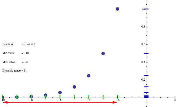
Before going there, let’s find a way of analyzing it and displaying dynamic range – first for the simplest case, no OETF, just plain 8bit storage of 8bit values.

Since 0 is “no signal”, I will use 1/256 as lowest representable signal (anything lower than that gets lost in quantization noise) and 1 as highest representable signal. If you can think of a better way – let me know in comments. To help me with that process, I created a Mathematica notebook.

Here is output showing numerical analysis of dynamic range:

Representation of EV stops in linear space is obviously exponential in nature and you can immediately see a problem with such naive encoding – many lower stops of exposure get “squished” in darks, while last 2 stops cover 3/4 of the range! Such linear encoding is extremely wasteful for logarithmic in nature signal and would result in quite large, unpleasant banding after quantization. Such “linear” values are unfortunately not perceptually linear. This is where gamma comes in, but before we proceed to analyze how it affects the dynamic range, let’s gave a look at some operations in EV / logarithmic space.

Exposure in EV space

First operation in EV space is trivial, it’s adjusting the exposure. Quite obviously, addition in logarithmic space is multiplication in linear space.

exp2(x+y) == exp2(x)*exp2(y)

Exposure operation does not modify dynamic range! It just shifts it in the EV scale. Let’s have a look:

Blue lines scale linearly, while green lines just shift – as expected.

Gamma in EV space

This is where things start to get interesting as most people don’t have intuition about logarithmic spaces – at least I didn’t have. Gamma is usually defined as a simple power function in linear space. What is interesting though is what happens when you try to convert it to EV space:

gamma(x,y) = pow(x, y)

log2(gamma(exp2(x),y)) == log2(exp2(x*y))

log2(exp2(x*y)) == x*y

Gamma operation becomes simple multiplication! This is a property that is actually used by GPUs to express a power operation through a series of exp2, madd and log2. However, if we stay in EV space, we only need the multiply part of this operation. Multiplication as a linear transform obviously preserves space linearity, just stretching it. Therefore gamma operation is essentially dynamic range compression / expansion operation!

You can see what it’s doing to original 8 bit dynamic range of 8 stops – it multiplies it by reverse of the gamma exponent.

Contrast

Gamma is a very useful operator, but when it increases dynamic range, it makes all values brighter than before; when decreasing dynamic range, it makes all of them darker. This comes from anchoring at zero (as 0 multiplied by any value will stay zero), which translates to “maximum” one in linear space. It is usually not desired property – when we talk about contrast, we want to make image more or less contrasty without adjusting overall brightness. We can compensate for it though! Just pick another, different anchor value – for example mid grey value.

Contrast is therefore quite similar to gamma – but we usually want to keep some other point fixed when dynamic range gets squished instead of 1 – for example linear middle gray 0.18.

contrast(x, y, midPoint) = pow(x,y) * midPoint / pow(midPoint, y)

How it all applies to local exposure

Hopefully, with this knowledge it’s clear why localized exposure works better to preserve local contrast, saturation and “punchiness” than either contrast or gamma operator – it moves parts of histogram (ones that were too dark / bright), but:

1. Does it only to the parts of the image / histogram that artist wanted, not affecting others like e.g. existing midtones.
2. Only shifts values (though movement range can vary!), instead of squishing / rescaling everything like gamma would do.

This property and contrast preservation is highly desired and preserves other properties as well – like saturation and “punchiness”.

EOTF vs OETF

Before talking about output functions, it’s important to distinguish between a function that’s used by display devices to transfer from electric signals (digital or analog), called EOTF – Electro Optical Transfer Function and the inverse of it, OETF, Opto-Electrical Transfer Function.

EOTF came a long way – from CRT displays and their power response to voltage that was seen as perceptually uniform in some viewing conditions.

While early rendering pipelines completely ignored gamma and happily used its perceptual linearity property and did output values directly to be raised to a gamma power by monitor, when starting to get more “serious” about things like working in linear spaces, we started to use inverse of this function, called OETF and this is what we use to encode signal for display in e.g. sRGB or Rec709 (and many more other curves like PQ).

While we don’t use CRTs anymore, such power encoding was proven to be very useful also on modern displays as it allows to encode more signal and this is why we still use them. There is even standard called BT1886 (it specifies only EOTF) that is designed to emulate gamma power look of old CRTs!

Monitor OETF gamma 2.2 encoding

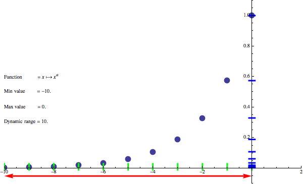
Equipped with that knowledge, we can get back to monitor 2.2 gamma. As EOTF is 2.2, OETF will be a gamma function of 1/2.2, ~0.45 and hopefully it’s now obvious that encoding from linear space to gamma space, we will have a dynamic range 2.2 * 8 == 17.6.

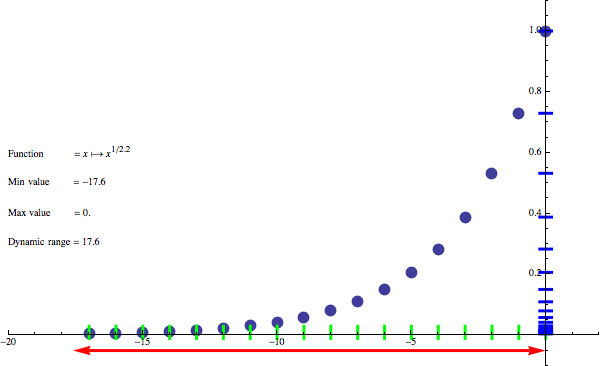
Now someone would ask – ok, hold on, I thought that monitors use a sRGB function, that is combination of a small, linear part and an exponent of 2.4!

Why I didn’t use precise sRGB? Because this function was designed to deliver average gamma 2.2, but have added linear part in smallest range to avoid numerical precision issues. So in this post instead of sRGB, I will be using gamma 2.2 to make things simpler.

What is worth noting here is that just gamma 2.2 of linear value encoded in 8 bits has huge dynamic range! I mean, potential to encode over 17 stops of exposure / linear values – should be enough? Especially that their distribution also gets better – note how more uniform is coverage of y axis (blue “ticks”) in the upper part. It still is not perfect, as it packs many more EV stops into shadows and puts most of the encoding range to upper values (instead of midtones), but we will fix it in a second.

Does this mean that OETF of gamma 2.2 allow TVs and monitors to display those 17.6 stops of exposure and we don’t need any HDR displays nor localized tonemapping? Unfortunately not. Just think about following question – how much information is really there between 1/256 and 2/256? How much those 2.2 EV stops mean to the observer? Quite possibly they won’t be even noticed! This is because displays have their own dynamic range (often expressed as contrast ratio) and depend on viewing conditions. Presentation by Timothy Lottes explained it very well.

But before I proceed with further analysis of how tonemapping curves change it and what gamma really does, I performed a small experiment with viewing conditions (let you be the judge if results are interesting and worth anything).

Viewing conditions

I wanted to do small experiment – compare an iPhone photo of the original image in my post about localized tonemapping (so the one with no localized tonemapping/exposure/contrast) on my laptop in perfect viewing conditions (isolated room with curtains):

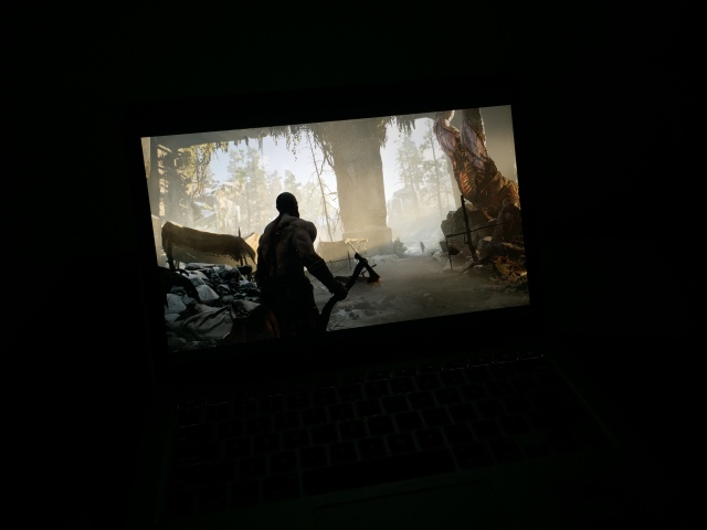
Poor dynamic range of the phone doesn’t really capture it, but it looked pretty good – with all the details preserved and lots of information in shadows. Interesting, HDR scene and shadows that look really dark, but full of detail and bright, punchy highlights. In such perfect viewing conditions, I really didn’t need any adjustments and the image and display looked “HDR” by themselves!

Second photo is in average/typical viewing conditions:

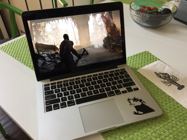
Whole image was still clear and readable, though what could be not visible here is that darks lost details; Image looks more contrasty (Bartleson-Breneman effect) and Kratos back was unreadable anymore.

Finally, same image taken outside (bright Californian sun around noon, but laptop maxed out on brightness!):

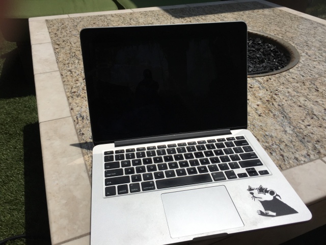
Yeah, almost invisible. This is with brightness adjustments (close to perception of very bright outdoor scene):

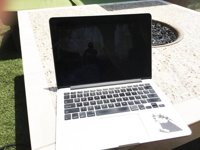
Not only image is barely visible and lost all the details, but also is overpowered with reflections of surroundings. Almost no gamma settings would be able to help such dynamic range and brightness.

I am not sure whether this artificial experiment shows it clearly enough, but depending on the viewing conditions image can look great and clear or barely visible at all.

My point is to emphasize what Timothy Lottes shown in his presentation – viewing conditions define the perceived dynamic range.

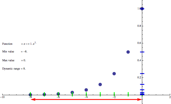
I tried to model it numerically – imagine that due to bright room and sunlight, you cannot distinguish anything below encoded 0.25. This is how dynamic range of such scene would look like:

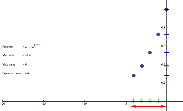
Not good at all, only 4.4 EV stops! And this is one of reasons why we might need some localized tonemapping.

Viewing conditions of EOTF / OETF

Viewing conditions and perception is also the reason for various gamma EOTF curves and their inverse. Rec709 EOTF transfer curve is different than sRGB transfer curve (average gamma of 2.4 vs 2.2) because of that – darker viewing conditions of HDTV require different contrast and reproduction.

Due to mentioned Bartleson-Breneman effect (we perceive more contrast, less dynamic range as surroundings get brighter) living room at night requires different EOTF than one for view conditions web content in standard office space (sRGB). Rec709 EOTF gamma will mean more contrast produced by the output device.

Therefore, using inverse of that function, OETF of Rec709 you can store 2.4*8 == 19.2 stops of exposure and the TV is supposed to display them and conditions are supposed to be good enough. This is obviously not always the case and if you tried to play console games in sunlit living room you know what I mean.

Gammas 2.2 and 2.4 aren’t only ones used – before standardizing sRGB and Rec709 different software and hardware manufacturers were using different values! You can find historical references to Apple Mac gammas 1.8 or 2.0 or crazy Gameboy extreme gammas of 3.0 or 4.0 (I don’t really understand this choice for Gameboys that are handheld and supposed to work in various conditions – if you know, let me and readers know in comments!).

“Adjust gamma until logo is barely visible”

Varying conditions are main reason for what you see in most games (especially on consoles!):

Sometimes it has no name and is called just a “slider”, sometimes gamma, sometimes contrast / brightness (incorrectly!), but it’s essentially way of correcting for imperfect viewing conditions. This is not the same as display gamma! It is an extra gamma that is used to reduce (or increase) the contrast for the viewing conditions.

It is about packing more EV stops into upper and midrange of the histogram (scaling and shifting right), more than expected by display before it turns it into linear values. So a contrast reduction / dynamic range compression operation as in brighter viewing conditions, viewer will perceive more contrast anyway.

It often is “good enough” but what in my opinion games usually do poorly is:

1. Often user sets it only once, but plays the game during different conditions! Set once, but then play same gam during day/night/night with lights on.
2. Purpose of it is not communicated well. I don’t expect full lecture on the topic, but at least explanation that it depends on brightness of the room where content is going to be viewed.

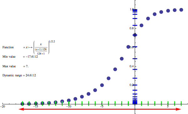
Let’s take our original “poor viewing conditions” graph and apply first 0.7 gamma (note: this additional gamma has nothing to do with the display EOTF! This is our “rendering intent” and knowledge about viewing conditions that are not part of the standard) on the linear signal before applying output transform, so:

(x^0.7)^(1/2.2) == x^(0.7/2.2)

A little bit better, ~1.42 more stops. 🙂 However, in good viewing conditions (like player of your game launching it at night), this will make image look less contrasty and much worse…

Tonemapping operators

From my analysis so far it doesn’t seem immediately obvious why we need some tonemapping curves / operators – after all we get relatively large dynamic range just with straight linear encoding in proper viewing conditions, right?

There are two problems:

1. First one is non-uniform distribution of data, biased towards last visible EV stops (values close to white) occupying most of the encoded range. We would probably want to have store most EV stops around middle values and larger range and have upper and lower range squishing many EV stops with smaller precision. So a non-uniform dynamic range scaling with most of precision bit range used for midtones.
2. Fixed cutoff value of 1.o defining such white point. It is highly impractical with HDR rendering, where while after exposure we can have most of values in midrange, we can also have lots of (sometimes extreme!) dynamic range in bright areas. This is true especially with physically based rendering and very glossy speculars or tiny emissive objects with extreme emitted radiance.

Methods presented so far don’t offer any solution for those very bright objects – we don’t want to reduce contrast or shift the exposure and we don’t want them to completely lose their saturation; we still want to perceive some details there.

This is where tonemapping curves come to play and show their usefulness. I will show some examples using good, old, Reinhard curve – mostly for its simplicity. By no means I recommend this curve, there are better alternatives!

There is a curve that probably every engine has implemented as a reference – Hable Uncharted tonemapping curve.

Another alternative is adapting either full ACES workflow – or cheaper (but less accurate; ACES RRT and ODT are not just curves and have some e.g. saturation preserving components!) approximating it like Kris Narkowicz proposed.

Finally, option that I personally find very convenient is nicely designed generic filmic tonemapping operator from Timothy Lottes.

I won’t focus here on them – instead try good, old Reinhard in simplest form – just for simplicity. It’s defined as simply:

tonemap(x) = x/(1+x)

It’s a curve that never reaches white point, so usually a rescaling correction factor is used (as division by tonemap(whitePoint) ).

Let’s have a look at Reinhard dynamic range and its distribution:

This looks great – we not only gained over 7 stops of exposure, have them tightly packed in brights without affecting midtones and darks too much, but also distribution of EV stops in final encoding looks almost perfect!

It also allows to distinguish (to some extent) details in objects that are way brighter than original value of EV 0 (after exposure) – like emissives, glowing particles, fire, bright specular reflections. Anything that is not “hotter” than 128 will get some distinction and representation.

As I mentioned, I don’t recommend this simplest Reinhard for anything other than firefly fighting in post effects or general variance reduction. There are better solutions (already mentioned) and you want to do many more things with your tonemapping – add some perceptual correction for darks contrast/saturation (“toe” of filmic curves), some minor channel crosstalk to prevent total washout of brights etc.

Summary

I hope that this post helped a bit with understanding of the dynamic range, exposure and EV logarithmic space, gamma functions and tonemapping. I have shown some graphs and numbers to help not only “visualize” impact of those operations, but also see how they apply numerically.

Perfect understanding of those concepts is in my opinion absolutely crucial for modern rendering pipelines and any future experiments with HDR displays.

If you want to play with this “dynamic range simulator” yourself, check the referenced Mathematica notebook!

.nb Matematica version

PDF version of the notebook

Edit: I would like to thank Jorge Jimenez for a follow up discussion that allowed me to make some aspects of my post regarding EOTF / OETF hopefully slightly clearer and more understandable.

References

http://renderwonk.com/publications/s2010-color-course/ SIGGRAPH 2010 Course: Color Enhancement and Rendering in Film and Game Production

http://gpuopen.com/gdc16-wrapup-presentations/  “Advanced Techniques and Optimization of HDR Color Pipelines”, Timothy Lottes.

http://filmicgames.com/archives/75 John Hable “Filmic Tonemapping Operators”

https://github.com/ampas/aces-dev Academy Color Encoding Standard

https://knarkowicz.wordpress.com/2016/01/06/aces-filmic-tone-mapping-curve/ ACES filmic tonemapping curve

http://graphicrants.blogspot.com/2013/12/tone-mapping.html Brian Karis “Tone-mapping”